Model Description

The model is expressed as a MILP or LP problem. Continuous variables include the individual unit dispatched power, the shedded load and the curtailed power generation. The binary variables are the commitment status of each unit. The main model features can be summarized as follows:

Variables

Sets

Name	Description
f	Fuel types
h	Hours
i	Time step in the current optimization horizon
l	Transmission lines between nodes
mk	{DA: Day-Ahead, 2U: Reserve up, 2D: Reserve Down}
n	Zones within each country (currently one zone, or node, per country)
p	Pollutants
t	Power generation technologies
tr	Renewable power generation technologies
u	Units
s	Storage units (including hydro reservoirs)
chp(u)	CHP units

Parameters

Name	Units	Description
AvailabilityFactor(u,i)	%	Percentage of nominal capacity available
CHPPowerLossFactor(u)	%	Power loss when generating heat
CHPPowerToHeat(u)	%	Nominal power-to-heat factor
CHPMaxHeat(chp)	MW	Maximum heat capacity of chp plant
CHPType	n.a.	CHP Type
CommittedInitial(u)	n.a.	Initial commitment status
CostFixed(u)	EUR/h	Fixed costs
CostLoadShedding(n,h)	EUR/MWh	Shedding costs
CostRampDown(u)	EUR/MW	Ramp-down costs
CostRampUp(u)	EUR/MW	Ramp-up costs
CostShutDown(u)	EUR/h	Shut-down costs
CostStartUp(u)	EUR/h	Start-up costs
CostVariableH(u,i)	EUR/MWh	Variable costs
Curtailment(n)	n.a.	Curtailment {binary: 1 allowed}
Demand(mk,n,i)	MW	Hourly demand in each zone
Efficiency(u)	%	Power plant efficiency
EmissionMaximum(n,p)	EUR/tP	Emission limit per zone for pollutant p
EmissionRate(u,p)	tP/MW	Emission rate of pollutant p from unit u
FlexibilityDown(u)	MW/h	Available fast shut-down ramping capacity
FlexibilityUp(u)	MW/h	Available fast start-up ramping capacity
Fuel(u,f)	n.a.	Fuel type used by unit u {binary: 1 u uses f}
LineNode(l,n)	n.a.	Line-zone incidence matrix {-1,+1}
LoadMaximum(u,h)	%	Maximum load for each unit
LoadShedding(n,h)	MW	Load that may be shed per zone in 1 hour
Location(u,n)	n.a.	Location {binary: 1 u located in n}
OutageFactor(u,h)	%	Outage factor (100 % = full outage) per hour
PartLoadMin(u)	%	Percentage of minimum nominal capacity
PowerCapacity(u)	MW	Installed capacity
PowerInitial(u)	MW	Power output before initial period
PowerMinStable(u)	MW	Minimum power for stable generation
PowerMustRun(u)	MW	Minimum power output
PriceTransmission(l,h)	EUR/MWh	Price of transmission between zones
RampDownMaximum(u)	MW/h	Ramp down limit
RampShutDownMaximum(u)	MW/h	Shut-down ramp limit
RampStartUpMaximum(u)	MW/h	Start-up ramp limit
RampUpMaximum(u)	MW/h	Ramp up limit
Reserve(t)	n.a.	Reserve provider {binary}
StorageCapacity(s)	MWh	Storage capacity (reservoirs)
StorageChargingCapacity(s)	MW	Maximum charging capacity
StorageChargingEfficiency(s)	%	Charging efficiency
StorageDischargeEfficiency(s)	%	Discharge efficiency
StorageInflow(s,h)	MWh	Storage inflows
StorageInitial(s)	MWh	Storage level before initial period
StorageMinimum(s)	MWh	Minimum storage level
StorageOutflow(s,h)	MWh	Storage outflows (spills)
StorageProfile(u,h)	MWh	Storage long-term level profile
Technology(u,t)	n.a.	Technology type {binary: 1: u belongs to t}
TimeDownInitial(u)	h	Hours down before initial period
TimeDownLeftInitial(u)	h	Time down remaining at initial time
TimeDownLeftJustStopped(u,i)	h	Time down remaining if started at time i
TimeDownMinimum(u)	h	Minimum down time
TimeDown(u,h)	h	Number of hours down
TimeUpInitial(u)	h	Number of hours up before initial period
TimeUpLeftInitial(u)	h	Time up remaining at initial time
TimeUpLeftJustStarted(u,i)	h	Time up remaining if started at time i
TimeUpMinimum(u)	h	Minimum up time
TimeUp(u,h)	h	Number of hours up
VOLL ()	EUR/MWh	Value of lost load

Optimization Variables

Name	Units	Description
Committed(u,h)	n.a.	Unit committed at hour h {1,0}
CostStartUpH(u,h)	EUR	Cost of starting up
CostShutDownH(u,h)	EUR	Cost of shutting down
CostRampUpH(u,h)	EUR	Ramping cost
CostRampDownH(u,h)	EUR	Ramping cost
CurtailedPower(n,h)	MW	Curtailed power at node n
Flow(l,h)	MW	Flow through lines
Heat(chp,h)	MW	Heat output by chp plant
HeatSlack(chp,h)	MW	Heat satisfied by other sources
MaxRamp2U(u,h)	MW/h	Maximum 15-min Ramp-up capbility
MaxRamp2D(u,h)	MW/h	Maximum 15-min Ramp-down capbility
Power(u,h)	MW	Power output
PowerMaximum(u,h)	MW	Power output
PowerMinimum(u,h)	MW	Power output
ShedLoad(n,h)	MW	Shed load
StorageInput(s,h)	MWh	Charging input for storage units
StorageLevel(s,h)	MWh	Storage level of charge
Spillage(s,h)	MWh	Spillage from water reservoirs
SystemCostD	EUR	Total system cost for one optimization period
LostLoadMaxPower(n,h)	MW	Deficit in terms of maximum power
LostLoadRampUp(u,h)	MW	Deficit in terms of ramping up for each plant
LostLoadRampDown(u,h)	MW	Deficit in terms of ramping down
LostLoadMinPower(n,h)	MW	Power exceeding the demand
LostLoadReserve2U(n,h)	MW	Deficit in reserve up

Optimisation model

The aim of this model is to represent with a high level of detail the short-term operation of large-scale power systems solving the so-called unit commitment problem. To that aim we consider that the system is managed by a central operator with full information on the technical and economic data of the generation units, the demands in each node, and the transmission network.

The unit commitment problem considered in this report is a simplified instance of the problem faced by the operator in charge of clearing the competitive bids of the participants into a wholesale day-ahead power market. In the present formulation the demand side is an aggregated input for each node, while the transmission network is modelled as a transport problem between the nodes (that is, the problem is network-constrained but the model does not include the calculation of the optimal power flows).

The unit commitment problem consists of two parts: i) scheduling the start-up, operation, and shut down of the available generation units, and ii) allocating (for each period of the simulation horizon of the model) the total power demand among the available generation units in such a way that the overall power system costs is minimized. The first part of the problem, the unit scheduling during several periods of time, requires the use of binary variables in order to represent the start-up and shut down decisions, as well as the consideration of constraints linking the commitment status of the units in different periods. The second part of the problem is the so-called economic dispatch problem, which determines the continuous output of each and every generation unit in the system. Therefore, given all the features of the problem mentioned above, it can be naturally formulated as a mixed-integer linear program (MILP).

Since our goal is to model a large European interconnected power system, we have implemented a so-called tight and compact formulation, in order to simultaneously reduce the region where the solver searches for the solution and increase the speed at which the solver carries out that search. Tightness refers to the distance between the relaxed and integer solutions of the MILP and therefore defines the search space to be explored by the solver, while compactness is related to the amount of data to be processed by the solver and thus determines the speed at which the solver searches for the optimum. Usually tightness is increased by adding new constraints, but that also increases the size of the problem (decreases compactness), so both goals contradict each other and a trade-off must be found.

Objective function

The goal of the unit commitment problem is to minimize the total power system costs (expressed in EUR in equation ), which are defined as the sum of different cost items, namely: start-up and shut-down, fixed, variable, ramping, transmission-related and load shedding (voluntary and involuntary) costs.

\[\begin{split}\begin{split} & min \sum _{u,n,i} \\ & \Big[ CostStartUp_{u,i} + CostShutDown_{u,i} + CostFixed_{u} \cdot Committed_{u,i} \\ & + CostVariable_{u,i} \cdot Power_{u,i} + CostRampUp_{u,i} + CostRampDown_{u,i} \\ & + PriceTransimission_{i,l} \cdot Flow_{i,l} + \left( CostLoadShedding_{i,n} \cdot ShedLoad_{i,n} \right) \\ & + \sum _{chp} CostHeatSlack_{chp,i} \cdot HeatSlack_{chp,i}) \\ & + \sum _{chp} CostVariable_{chp,i} \cdot CHPPowerLossFactor_{chp} \cdot Heat_{chp,i}) \\ & + VOLL_{Power} \cdot \left( LostLoadMaxPower_{i,n} + LostLoadMinPower_{i,n} \right) \\ & + VOLL_{Reserve} \cdot \left( LostLoadReserve2U_{i,n} + LostLoadReserve2D_{i,n} \right) \\ & + VOLL_{Ramp} \cdot \left( LostLoadRampUp_{u,i} + LostLoadRampDown_{u,i} \right) \Big] \end{split}\end{split}\]

The costs can be broken down as:

• Fixed costs: depending on whether the unit is on or off.
• Variable costs: stemming from the power output of the units.
• Start-up costs: due to the start-up of a unit.
• Shut-down costs: due to the shut-down of a unit.
• Ramp-up: emerging from the ramping up of a unit.
• Ramp-down: emerging from the ramping down of a unit.
• Load shed: due to necessary load shedding.
• Transmission: depending of the flow transmitted through the lines.
• Loss of load: power exceeding the demand or not matching it, ramping and reserve.

The variable production costs (in EUR/MWh), are determined by fuel and emission prices corrected by the efficiency (which is considered to be constant for all levels of output in this version of the model) and the emission rate of the unit (equation ):

\[\mathit{CostVariable}_{u,h}=\]\[\mathit{Markup}_{u,h} + \sum _{n,f}\left(\frac{\mathit{Fuel}_{u,f} \cdot \mathit{FuelPrice}_{n,f,h} \cdot \mathit{Location}_{u,n}}{\mathit{Efficiency}_u}\right)\]\[ + \sum _p\left(\mathit{EmissionRate}_{u,p} \cdot \mathit{PermitPrice}_p\right)\]

The variable cost includes an additional mark-up parameter that can be used for calibration and validation purposes.

The start-up and shut-down costs are positive variables, active when the commitment status between two consecutive time periods is modified:

\[i=1:\]\[\mathit{CostStartUp}_{u,i} \geq \mathit{CostStartUp}_u \cdot \left(\mathit{Committed}_{u,i}-\mathit{CommittedInitial}_u\right)\]\[\mathit{CostShutDown}_{u,i} \geq \mathit{CostShutDown}_u \cdot (\mathit{CommittedInitial}_u-\mathit{Committed}_{u,i})\]\[\begin{split}i>1:\end{split}\]\[\mathit{CostStartUp}_{u,i} \geq \mathit{CostStartUp}_u \cdot \left(\mathit{Committed}_{u,i}-\mathit{Committed}_{u,i-1}\right)\]\[\mathit{CostShutDown}_{u,i} \geq \mathit{CostShutDown}_u \cdot (\mathit{Committed}_{u,i-1}-\mathit{Committed}_{u,i})\]

In the previous equation, as in some of the following, a distinction is made between the equation for the first and subsequent periods. The equation for the first period takes into account the commitment status of the unit before the beginning of the simulation, which is part of the information fed into the model.

Ramping costs are computed in the same manner:

\[i=1:\]\[\mathit{CostRampUp}_{u,i} \geq \mathit{CostRampUp}_u \cdot \left(\mathit{Power}_{u,i}-\mathit{PowerInitial}_u\right)\]\[\mathit{CostRampDown}_{u,i} \geq \mathit{CostRampDown}_u \cdot (\mathit{PowerInitial}_u-\mathit{Power}_{u,i})\]\[\begin{split}i>1:\end{split}\]\[\mathit{CostRampUp}_{u,i} \geq \mathit{CostRampUp}_u \cdot \left(\mathit{Power}_{u,i}-\mathit{Power}_{u,i-1}\right)\]\[\mathit{CostRampDown}_{u,i} \geq \mathit{CostRampDown}_u \cdot (\mathit{Power}_{u,i-1}-\mathit{Power}_{u,i})\]

It should be noted that in case of start-up and shut-down, the ramping costs are added to the objective function. Using start-up, shut-down and ramping costs at the same time should therefore be performed with care.

In the current formulation all other costs (fixed and variable costs, transmission costs, load shedding costs) are considered as exogenous parameters.

As regards load shedding, the model considers the possibility of voluntary load shedding resulting from contractual arrangements between generators and consumers. Additionally, in order to facilitate tracking and debugging of errors, the model also considers some variables representing the capacity the system is not able to provide when the minimum/maximum power, reserve, or ramping constraints are reached. These lost loads are a very expensive last resort of the system used when there is no other choice available. The different lost loads are assigned very high values (with respect to any other costs). This allows running the simulation without infeasibilities, thus helping to detect the origin of the loss of load. In a normal run of the model, without errors, all these variables are expected to be equal to zero.

Demand-related constraints

The main constraint to be met is the supply-demand balance, for each period and each zone, in the day-ahead market (equation ). According to this restriction, the sum of all the power produced by all the units present in the node (including the power generated by the storage units), the power injected from neighbouring nodes, and the curtailed power from intermittent sources is equal to the load in that node, plus the power consumed for energy storage, minus the load interrupted and the load shed.

\[\sum _u\left(\mathit{Power}_{u,i} \cdot \mathit{Location}_{u,n}\right)\]\[ + \sum _l\left(\mathit{Flow}_{l,i} \cdot \mathit{LineNode}_{l,n}\right)\]\[=\mathit{Demand}_{\mathit{DA},n,h} + \sum _r\left(\mathit{StorageInput}_{s,h} \cdot \mathit{Location}_{s,n}\right)\]\[ -\mathit{ShedLoad}_{n,i}\]\[ - \mathit{LostLoadMaxPower}_{n,i} + \mathit{LostLoadMinPower}_{n,i}\]

Besides that balance, the reserve requirements (upwards and downwards) in each node must be met as well. In Dispa-SET, the reserve requirements are defined as an aggregation of secondary and tertiary reserves, which are typically brought online in periods shorter than an hour, the time step of this model. Therefore, additional equations and constraints are defined to account for the up/down ramping requirements, by computing the ability of each unit to adapt its power output within a period of 15 min.

For each power plant, the ability to increase its power (in MW/h) is the ramp-up capability if it is already committed or the nominal power if it is stopped and its starting time is lower than 15 minutes. This is to take into account that fast starting units could provide reserve (hydro units for secondary reserve, gas turbine for tertiary reserve).

\[\mathit{MaxRamp}2U_{u,i}\]\[\leq \mathit{RampUpMaximum}_u \cdot \mathit{Committed}_{u,i}\]\[+ \mathit{FlexibilityUp}_u \cdot \left(1-\mathit{Committed}_{u,i} \right)\]

where FlexibilityUp is the maximum flexibility (in MW/h) that can be provided by the unit in 15 min in case of cold start:

\[If ~ \mathit{RampStartUpMaximum}_u \geq \mathit{PowerMinStable}_u \cdot 4\]\[Then ~ \mathit{FlexibilityUp}_u = \mathit{RampStartUpMaximum}_u\]\[Else ~ \mathit{FlexibilityUp}_u = 0\]

where the factor 4 is used to convert the ramping rate from MW/15min to MW/h.

The maximum ramping rate is also limited by the available capacity margin between current and maximum power output:

\[\mathit{MaxRamp2U}_{u,i} \leq (\mathit{PowerCapacit}y_u \cdot \mathit{AvailabilityFactor}_{u,i}\]\[ \cdot (1-\mathit{OutageFactor}_{u,i})-\mathit{Power}_{u,i}) \cdot 4\]

The same applies to the 15 min ramping down capabilities:

\[\mathit{MaxRamp}2D_{u,i}\]\[ \leq \mathit{max}\left(\mathit{RampDownMaximu}m_u,\mathit{Flexibility}\mathit{Down}_u\right) \cdot \mathit{Committed}_{u,i}\]

The parameter FlexibilityDown is defined as the maximum ramp down rate at which the unit can shut down in 15 minutes. In case the unit cannot be shut-down in 15 minutes (and only in this case) the maximum ramping down capability is limited by the capacity margin between actual and minimum power:

\[\begin{split} If \mathit{RampShutDownMaximu}m_u<\mathit{PowerMinStabl}e_u \cdot 4 :\end{split}\]\[ \mathit{MaxRamp}2D_{u,i} \leq \left(\mathit{Power}_{u,i}-\mathit{PowerMinStable}_u \cdot \mathit{Committed}_{u,i}\right) \cdot 4\]\[ Else :\]\[\mathit{MaxRamp}2D_{u,i} \leq \mathit{Power}_{u,i} \cdot 4\]

The reserve requirements are defined by the users. In case no input is provided a default formula is used to evaluate the needs for secondary reserves as a function of the maximum expected load for each day. The default formula is described by:

\[\mathit{Demand}_{2U,n,i}=\sqrt{10 \cdot \underset h{\mathit{max}}\left(\mathit{Demand}_{\mathit{DA},n,h}\right) + 150^2}-150\]

Downward reserves are defined as 50% of the upward margin:

\[\mathit{Demand}_{2D,n,h}=0.5 \cdot \mathit{Demand}_{2U,n,h}\]

The reserve demand should be fulfilled at all times by all the plants allowed to participate in the reserve market:

\[\mathit{Demand}_{2U,n,h}\]\[ \leq \sum _{u,t}\left(\mathit{MaxRamp}2U_{u,i} \cdot \mathit{Technology}_{u,t} \cdot \mathit{Reserv}e_t \cdot \mathit{Locatio}n_{u,n}\right)\]\[+ \mathit{LostLoadReserve2UH}_{n,i}\]

The same equation applies to downward reserve requirements (2D).

Power output bounds

The minimum power output is determined by the must-run or stable generation level of the unit if it is committed:

\[\mathit{Power}\mathit{MustRun}_{u,i} \cdot \mathit{Committed}_{u,i}\]\[ \leq \mathit{Power}_{u,i}\]

On the other hand, the output is limited by the available capacity, if the unit is committed:

\[\mathit{Power}_{u,i}\]\[ \leq \mathit{PowerCapacity}_u \cdot \mathit{AvailabilityFactor}_{u,i}\]\[ \cdot (1-\mathit{OutageFactor}_{u,i}) \cdot \mathit{Committed}_{u,i}\]

The availability factor is used for renewable technologies to set the maximum time-dependent generation level. It is set to one for the traditional power plants. The outage factor accounts for the share of unavailable power due to planned or unplanned outages.

The power output in a given period also depends on the output levels in the previous and the following periods and on the ramping capabilities of the unit. If the unit was down, the ramping capability is given by the maximum start up ramp, while if the unit was online the limit is defined by the maximum ramp up rate. Those bounds are given with respect to the previous time step by the equation :

\[i=1:\]\[\mathit{Power}_{u,i} \leq\]\[\mathit{PowerInitial}_u\]\[ + \mathit{CommittedInitial}_u \cdot \mathit{RampUpMaximum}_u\]\[ + \left(1-\mathit{CommittedInitial}_u\right) \cdot \mathit{RampStartUpMaximum}_u\]\[ + \mathit{LostLoadRampUp}_{u,i}\]\[\begin{split}i>1:\end{split}\]\[\mathit{Power}_{u,i} \leq\]\[\mathit{Power}_{u,i-1}\]\[ + \mathit{Committed}_{u,i-1} \cdot \mathit{RampUpMaximum}_u\]\[ + \left(1-\mathit{Committed}_{u,i-1}\right) \cdot \mathit{RampStartUpMaximum}_u\]\[ + \mathit{LostLoadRampUp}_{u,i}\]

Where the LoadMaximum parameter is calculated taking into account the availability factor and the outage factor:

\[\mathit{LoadMaximum}_{u,h}=\mathit{AvailabilityFactor}_{u,h} \cdot (1-\mathit{OutageFactor}_{u,h})\]

Similarly, the ramp down capability is limited by the maximum ramp down or the maximum shut down ramp rate:

\[i=1:\]\[\mathit{PowerInitial}_u-\mathit{Power}_{u,i} \leq\]\[\mathit{Committed}_{u,i} \cdot \mathit{RampDownMaximum}_u\]\[ + \left(1-\mathit{Committed}_{u,i}\right) \cdot \mathit{RampShutDownMaximum}_u\]\[ + \mathit{LostLoadRampDown}_{u,i}\]\[\begin{split}i>1:\end{split}\]\[\mathit{Power}_{u,i-1}-\mathit{Power}_{u,i} \leq\]\[\mathit{Committed}_{u,i} \cdot \mathit{RampDownMaximum}_u\]\[ + \left(1-\mathit{Committed}_{u,i}\right) \cdot \mathit{RampShutDownMaximum}_u\]\[ + \mathit{LostLoadRampDown}_{u,i}\]

Minimum up and down times

The operation of the generation units is also limited as well by the amount of time the unit has been running or stopped. In order to avoid excessive ageing of the generators, or because of their physical characteristics, once a unit is started up, it cannot be shut down immediately. Reciprocally, if the unit is shut down it may not be started immediately.

That is, the value of the time counter with respect to the minimum up time and down times determines the commitment status of the unit. In order to model theses constraints linearly, it is necessary to keep track of the number of hours the unit must be online at the beginning of the simulation:

\[\mathit{TimeUpLeftInitial}_u =\]\[\mathit{min}\left\{N,\left(\mathit{TimeUpMinimum}_u - \mathit{TimeUpInitial}_u\right) \cdot \mathit{CommittedInitial}_u\right\}\]

where N is the number of time steps in the current optimisation horizon.

If the unit is initially started up, it has to remain committed until reaching the minimum up time:

\[\sum _{i=1}^{\mathit{TimeUpLeftInitial}_u}\left(1-\mathit{Committed}_{u,i}\right)=0\]

If the unit is started during the considered horizon, the time it has to remain online is TimeUpMinimum, but cannot exceed the time remaining in the simulated period. This is expressed in equation and is pre-calculated for each time step of the period.

\[\mathit{TimeUpLeftJustStarted}_{u,i}=\]\[\mathit{min}\left\{N -i + 1,\mathit{TimeUpMinimum}_u\right\}\]

The equation imposing the unit to remain committed is written:

\[ i=1:\]\[ \sum _{\mathit{ii}=i}^{i + \mathit{TimeUpLeftJustStarted}_{u,i}-1}\mathit{Committed}_{u,\mathit{ii}} \geq\]\[ \mathit{TimeUpLeftJustStarted}_{u,i} \cdot \left(\mathit{Committed}_{u,i}-\mathit{CommittedInitial}_u\right)\]\[\begin{split} i>1:\end{split}\]\[ \sum _{\mathit{ii}=i}^{i + \mathit{TimeUpLeftJustStarted}_u-1}\mathit{Committed}_{u,\mathit{ii}} \geq\]\[\mathit{TimeUpLeftJustStarted}_{u,i} \cdot \left(\mathit{Committed}_{u,i}-\mathit{Committed}_{u,i-1}\right)\]

The same method can be applied to the minimum down time constraint:

\[\mathit{TimeDownLeft}_u =\]\[\mathit{min}\{N,(\mathit{TimeDownMinimum}_u-\mathit{TimeDownInitial}_u)\]\[\cdot (1-\mathit{CommittedInitial}_u)\}\]

Related to the initial status of the unit:

\[\sum _{i=1}^{\mathit{TimeDownLeft}_u}\mathit{Committed}_{u,i}=0\]

The TimeDownLeftJustStopped parameter is computed by:

\[\mathit{TimeDownLeftJustStopped}_{u,i} =\]\[\mathit{min}\left\{N - i + 1,\mathit{TimeDownMinimum}_u\right\}\]

Finally, the equation imposing the time the unit has to remain de-committed is defined as:

\[i=1:\]\[\sum _{\mathit{ii}=i}^{i + \mathit{TimeDownLeftJustStopped}_{i,u}-1}\left(1-\mathit{Committed}_{u,i}\right) \geq\]\[\mathit{TimeDownLeftJustStopped}_{u,i} \cdot \left(\mathit{CommittedInitial}_u-\mathit{Committed}_{u,i}\right)\]\[\begin{split}i>1:\end{split}\]\[\sum _{\mathit{ii}=i}^{i + \mathit{TimeDownLeftJustStopped}_u-1}\left(1-\mathit{Committed}_{u,i}\right) \geq\]\[\mathit{TimeDownLeftJustStopped}_{u,i} \cdot \left(\mathit{Committed}_{u,i-1}-\mathit{Committed}_{u,i}\right)\]

This formulation avoids the use of additional binary variables to describe the start-up and shut-down of each unit.

Storage-related constraints

Generation units with energy storage capabilities (mostly large hydro reservoirs and pumped hydro storage units) must meet additional restrictions related to the amount of energy stored. Storage units are considered to be subject to the same constraints as non-storage power plants. In addition to those constraints, storage-specific restrictions are added for the set of storage units (i.e. a subset of all units). These restrictions include the storage capacity, inflow, outflow, charging, charging capacity, charge/discharge efficiencies, etc. Discharging is considered as the standard operation mode and is therefore linked to the Power variable, common to all units.

The first constrain imposes that the energy stored by a given unit is bounded by a minimum value:

\[\mathit{StorageMinimum}_s \leq \mathit{StorageLevel}_{s,i}\]

In the case of a storage unit, the availability factor applies to the charging/discharging power, but also to the storage capacity. The storage level is thus limited by:

\[\mathit{StorageLevel}_{s,i} \leq \mathit{StorageCapacity}_s \cdot \mathit{AvailabilityFactor}_{s,i}\]

The energy added to the storage unit is limited by the charging capacity. Charging is allowed only if the unit is not producing (discharging) at the same time (i.e. if Committed, corresponding to the {textquotedbl}normal{textquotedbl} mode, is equal to 0).

\[\mathit{StorageInput}_{s,i} \leq \mathit{StorageChargingCapacity}_s\]\[\cdot \mathit{AvailabilityFactor}_{s,i} \cdot (1-\mathit{Committed}_{s,i})\]

Discharge is limited by the level of charge of the storage unit:

\[\frac{\mathit{Power}_{i,s}}{\mathit{StorageDischargeEfficienc}y_s} + \mathit{StorageOutflow}_{s,i}\]\[+ \mathit{Spillage}_{s,i} -\mathit{StorageInflow}_{s,i}\]\[\leq \mathit{StorageLevel}_{s,i}\]

Charge is limited by the level of charge of the storage unit:

\[\mathit{StorageInput}_{s,i} \cdot \mathit{StorageChargingEfficienc}y_s\]\[- \mathit{StorageOutflow}_{s,i} - \mathit{Spillage}_{s,i}\]\[+ \mathit{StorageInflow}_{s,i}\]\[\leq \mathit{StorageCapacity}_s-\mathit{StorageLevel}_{s,i}\]

Besides, the energy stored in a given period is given by the energy stored in the previous period, net of charges and discharges:

\[i=1:\]\[\mathit{StorageLevelInitial}_s + \mathit{StorageInflow}_{s,i}\]\[+ \mathit{StorageInput}_{s,i} \cdot \mathit{StorageChargingEfficiency}_s\]\[= \mathit{StorageLevel}_{s,i} + \mathit{StorageOutflow}_{s,i} + \frac{\mathit{Power}_{s,i}}{\mathit{StorageDischargeEfficienc}y_s}\]\[\begin{split}i>1:\end{split}\]\[\mathit{StorageLevel}_{s,i-1} + \mathit{StorageInflow}_{s,i}\]\[+ \mathit{StorageInput}_{s,i} \cdot \mathit{StorageChargingEfficiency}_s\]\[= \mathit{StorageLevel}_{s,i} + \mathit{StorageOutflow}_{s,i} + \frac{\mathit{Power}_{s,i}}{\mathit{StorageDischargeEfficienc}y_s}\]

Some storage units are equiped with large reservoirs, whose capacity at full load might be longer than the optimisation horizon. Therefore, a minimum level constraint is required for the last hour of the optimisation, which otherwise wouls systematically tend to empty the reservoir as much a possible. An exogenous minimum profile is thus provided and the following constraint is applied:

\[\mathit{StorageLevel}_{s,N} \geq min( \mathit{StorageProfile}_{s,N}\]\[\cdot \mathit{AvailabilityFactor}_{s,N} \cdot \mathit{StorageCapacity}_{s},\]\[\mathit{StorageLevel}_{s,0} + \sum\limits_{i=1}^N InFlows_{s,i} )\]

where StorageProfile is a non-dimensional minimum storage level provided as an exogenous input. The minimum is taken to avoid unfeasibilities in case the provided inflows are not sufficient to comply with the imposed storage level at the end of the horizon.

Heat production constraints (CHP plants only)

In DispaSET Power plants can be indicated as CHP satisfying one heat demand. Heat Demand can be covered either by a CHP plant or by alternative heat supply options (Heat Slack).

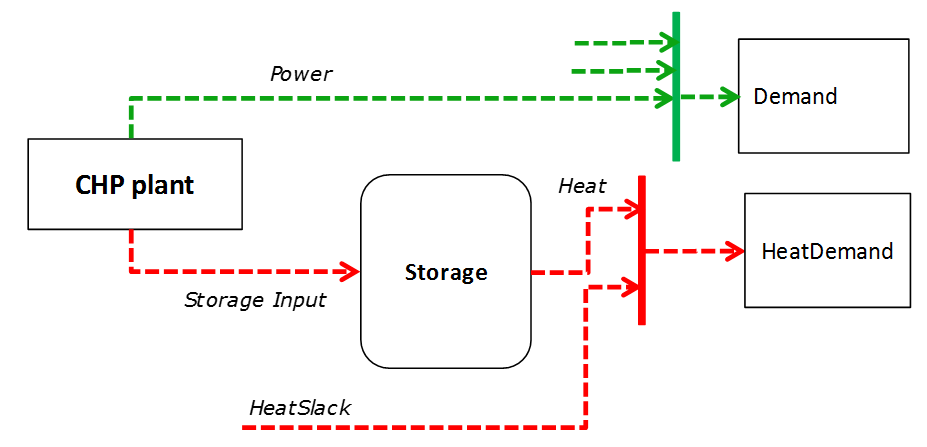
The following two heat balance constraints are used for any CHP plant type.

\[Heat(chp,i) + HeatSlack(chp,i) = HeatDemand(chp,i)\]

\[StorageInput_{chp,i} \leq CHPMaxHeat_{chp}\]

The constraints between heat and power production differ for each plant design and explained within the following subsections.

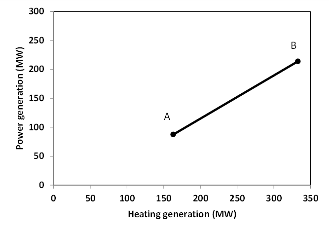
Steam plants with Backpressure turbine

This options includes steam-turbine based power plants with a backpressure turbine. The feasible operating region is between AB. The slope of the line is the heat to power ratio.

\[Power_{chp,i} = StorageInput_{chp,i} \cdot CHPPowerToHeat_{chp}\]

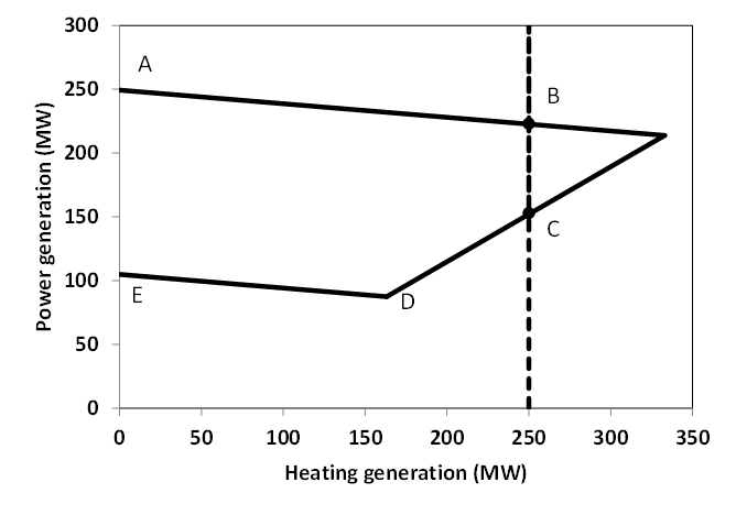
Steam plants with Extraction/condensing turbine

This options includes steam-turbine based power plants with an extraction/condensing turbine. The feasible operating region is within ABCDE. The vertical dotted line BC corresponds to the minimum condensation line (as defined by CHPMaxHeat). The slope of the DC line is the heat to power ratio and the slope of the AB line is the inverse of the power penalty ratio.

\[Power_{chp,i} \geq StorageInput_{chp,i} \cdot CHPPowerToHeat_{chp}\]

\[Power_{chp,i} \leq PowerCapacity_{chp} -\]\[StorageInput_{chp,i} \cdot CHPPowerLossFactor_{chp}\]

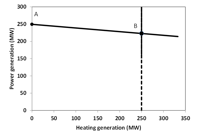
Power plant coupled with any power to heat option

This option includes power plants coupled with resistance heater or heat pumps. The feasible operating line is between AB. The slope of the line is the inverse of the COP or efficiency. The vertical dotted line corresponds to the heat pump (or resistance heater) thermal capacity (as defined by CHPMaxHeat)

\[Power_{chp,i} = PowerCapacity_{chp} - StorageInput_{chp,i} \cdot CHPPowerLossFactor_{chp}\]

Heat Storage

Heat storage is modeled in a similar way as electric storage as follows:

Heat Storage balance:

\[i=1:\]\[ StorageInitial_{chp} +StorageInput_{chp,i} =\]\[ StorageLevel_{chp,i} +Heat_{chp,i} + StorageSelfDischarge_{chp} \cdot StorageLevel_{chp,i}/24\]\[\begin{split}i>1:\end{split}\]\[+StorageLevel_{chp,i-1} +StorageInput_{chp,i} =\]\[StorageLevel_{chp,i} +Heat_{chp,i} + StorageSelfDischarge_{chp} \cdot StorageLevel_{chp,i}/24\]

Storage level must be above a minimum and below storage capacity:

\[StorageMinimum_{chp} \leq StorageLevel_{chp,i} \leq StorageCapacity_{chp}\]

Emission limits

The operating schedule also needs to take into account any cap on the emissions (not only CO2) from the generation units existing in each node:

\[\sum _u\left(\mathit{Power}_{u,i} \cdot \mathit{EmisionRate}_{u,p} \cdot \mathit{Location}_{u,n}\right)\]\[\leq \mathit{EmisionMaximum}_{n,p}\]

It is important to note that the emission cap is applied to each optimisation horizon: if a rolling horizon of one day is adopted for the simulation, the cap will be applied to all days instead of the whole year.

Network-related constraints

The flow of power between nodes is limited by the capacities of the transmission lines:

\[\mathit{FlowMinimum}_{l,i} \leq \mathit{Flow}_{l,i}\]\[\mathit{Flow}_{l,i} \leq \mathit{FlowMaximum}_{l,i}\]

In this model a simple Net Transfer Capacity (NTC) between countries approach is followed. No DC power flow or Locational Marginal Pricing (LMP) model is implemented.

Curtailment

If curtailment of intermittent generation sources is allowed in one node, the amount of curtailed power is bounded by the output of the renewable (tr) units present in that node:

\[\mathit{CurtailedPower}_{n,i}\]\[\leq \sum _{u,\mathit{tr}}\left(\mathit{Power}_{u,i} \cdot \mathit{Technology}_{u,\mathit{tr}} \cdot \mathit{Location}_{u,n}\right) \cdot \mathit{Curtailment}_n\]

Load shedding

If load shedding is allowed in a node, the amount of shed load is limited by the shedding capacity contracted on that particular node (e.g. through interruptible industrial contracts)

\[\mathit{ShedLoad}_{n,i} \leq \mathit{LoadShedding}_n\]

Rolling Horizon

The mathematical problem described in the previous sections could in principle be solved for a whole year split into time steps of one hour, but with all likelihood the problem would become extremely demanding in computational terms when attempting to solve the model with a realistically sized dataset. Therefore, the problem is split into smaller optimization problems that are run recursively throughout the year.

The following figure shows an example of such approach, in which the optimization horizon is one day, with a look-ahead (or overlap) period of one day. The initial values of the optimization for day j are the final values of the optimization of the previous day. The look-ahead period is modelled to avoid issues related to the end of the optimization period such as emptying the hydro reservoirs, or starting low-cost but non-flexible power plants. In this case, the optimization is performed over 48 hours, but only the first 24 hours are conserved.

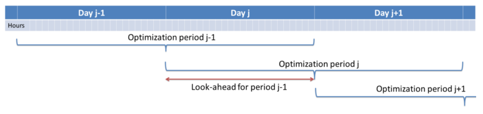
Although the previous example corresponds to an optimization horizon and an overlap of one day, these two values can be adjusted by the user in the Dispa-SET configuration file. As a rule of thumb, the optimization horizon plus the overlap period should as least twice the maximum duration of the time-dependent constraints (e.g. the minimum up and down times). In terms of computational efficiency, small power systems can be simulated with longer optimization horizons, while larger systems should reduce this horizon, the minimum being one day.

Power plant clustering

For computational efficiency reasons, it is useful to cluster some of the original units into larger units. This reduces the number of continuous and binary variables and can, in some conditions, be performed without significant loss of simulation accuracy.

The clustering occurs at the beginning of the pre-processing phase (i.e. the units in the Dispa-SET database do not need to be clustered).

In Dispa-SET, different clustering options are availble and can be automatically generated from the same input data. They are described in the two next sections.

MILP clustering

In this formulation, the units that are either very small or very flexible are aggregated into larger units. Some of these units (e.g. the turbojets) indeed present a low capacity or a high flexibility: their output power does not exceed a few MW and/or they can reach full power in less than 15 minutes (i.e. less than the simulation time step). For these units, a unit commitment model with a time step of 1 hour is unnecessary and computationally inefficient. They are therefore merged into one single, highly flexible unit with averaged characteristics.

The condition for the clustering of two units is a combination of subconditions regarding their type, maximum power, flexiblity and technical similarities. They are summarized in the figure below (NB: the thresholds are for indicative purpose only, they can be user-defined).

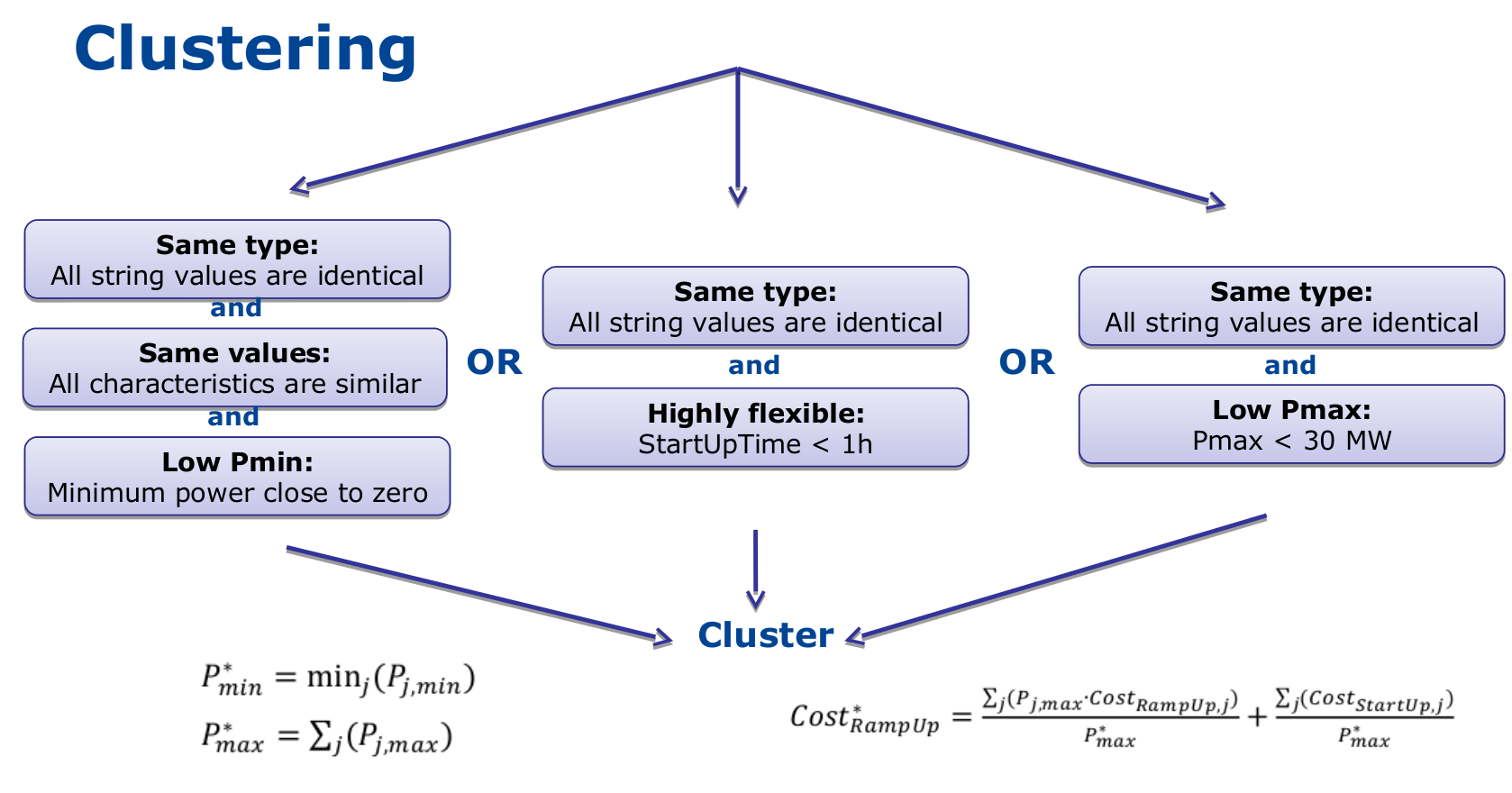
When two units are clustered, the minimum and maximum capacities of new aggregated units (indicated by the star) are given by:

\[P_{min}^* = min(P_{j,min})\]

\[P_{max}^* = \sum_j (P_{j,min})\]

The last equation is also applied for the storage capacity or for the storage charging power.

The unit marginal (or variable cost) is given by:

\[Cost_{Variable}^* = \frac{\sum_j ( P_{j,max} \cdot Cost_{Variable,j} )}{P_{max}^*}\]

The start-up/shut-down costs are transformed into ramping costs (example with ramp-up):

\[Cost_{RampUp}^* = \frac{\sum_j ( P_{j,max} \cdot Cost_{RampUp,j} )}{P_{max}^*} + \frac{\sum_j ( Cost_{StartUp,j} )}{P_{max}^*}\]

Other characteristics, such as the plant efficiency, the minimum up/down times or the CO2 emissions are computed as a weighted averaged:

\[Efficiency^* = \frac{\sum_j ( P_{j,max} \cdot Efficiency_{j} )}{P_{max}^*}\]

It should be noted that only very similar units are aggregated (i.e. their quantitative characteristics should be similar), which avoids errors due to excessive aggregation.

LP clustering

Dispa-SET provides the possibility to generate the optimisation model as an LP problem (i.e. withtout the binary variables). In that case, the following constraints are removed since they can only be expressed in an MILP formulation:

• Minimum up and down times
• Start-up costs
• Minimum stable load

Since the start-up of individual units is not considered anymore, it is not useful to disaggrate them in the optimisation. All units of a similar technology, fuel and zone can be aggregated into a single unit using the equations proposed in the previous section.

References

[1]	Quoilin, S., Hidalgo Gonzalez, I., & Zucker, A. (2017). Modelling Future EU Power Systems Under High Shares of Renewables: The Dispa-SET 2.1 open-source model. Publications Office of the European Union.

[2]	Quoilin, S., Nijs, W., Hidalgo, I., & Thiel, C. (2015). Evaluation of simplified flexibility evaluation tools using a unit commitment model. IEEE Digital Library.

[3]	Quoilin, S., Gonzalez Vazquez, I., Zucker, A., & Thiel, C. (2014). Available technical flexibility for balancing variable renewable energy sources: case study in Belgium. Proceedings of the 9th Conference on Sustainable Development of Energy, Water and Environment Systems.