Getting Started
This short tutorial describes the main steps to get a practical example of Dispa-SET running.
Prerequisites
Install Python 3.7, with full scientific stack. The Anaconda distribution is recommended since it comprises all the required packages. If Anaconda is not used, the following libraries and their dependencies should be installed manually:
- future >= 0.15
- click >= 3.3
- numpy>=1.10
- scipy>=0.15
- matplotlib>=1.5.1
- pandas>= 0.19
- xlrd >= 0.9
- pickle
- pyyaml >= 5.1
- pytest
Using Dispa-SET:
Dispa-SET is primarily designed to run with GAMS and therefore requires GAMS to be installed with a valid user licence. Currently, only the 64-bit version of GAMS is supported in Dispa-SET!
The GAMS api for python has been pre-compiled in the “Externals” folder and is usable for Windows 64 bit systems. If the pre-compiled binaries are not available or could not be loaded, they must be installed manually using following command in the Anaconda prompt:
pip install gdxcc gamsxcc optcc
Alternatively, the gams python api can also be compiled from the source provided in the GAMS installation folder (e.g. “C:\GAMS\win64\24.3\apifiles\Python\api”):
python setup.py install
NB: For Windows users, the manual api compilation might require the installation of a C++ compiler for Python. This corresponds to the typical error message: “Unable to find vcvarsall.bat”. This can be solved by installing the freely available “Microsoft Visual C++ Compiler for Python”. In some cases the path to the compiler must be added to the PATH windows environment variable (e.g. C:Program FilesCommon FilesMicrosoftVisual C++ for Python9.0)
The api requires the path to the gams installation folder. The “get_gams_path()” function of dispa-set performs a system search to automatically detect this path. It case it is not successful, the user is prompted for the proper installation path.
Step-by-step example of a Dispa-SET run
This section describes the pre-processing and the solving phases of a Dispa-SET run. Three equivalent methods are described in the next sections:
- Using the command line interface
- Using the Dispa-SET API
- Using GAMS
1. Using the command line interface
Dispa-SET can be run from the command line. To that aim, open a terminal window and change de directory to the Dispa-SET root folder.
1.0. Install Dispa-SET and the required dependencies
Use the following commands in a terminal (Anaconda prompt in Windows):
conda env create  # Automatically creates environment based on environment.yml
conda activate dispaset
pip install -e . # Install editable local version
The above commands create a dedicated environment so that your anconda configuration remains clean from the required dependencies installed. If preferred, the Gams libraries can also be installed without creating a dedicated environment. In that case, replace the above commands with these ones:
pip install gamsxcc gdxcc optcc
python setup.py install
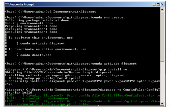
To check that everything runs fine, you can build and run a test case by typing:
dispaset -c ConfigFiles/ConfigTest.xlsx build simulate
1.1. Check the configuration file
Dispa-SET runs are defined in dedicated excel configuration files stored in the “ConfigFiles” folder. The configuration file “ConfigTest.xlsx” is provided for testing purposes. It generates a 10-days optimisation using data relative a fictitious power system composed of two zones Z1 and Z2.
1.2. Pre-processing
From the command line, specify the configuration file to be used as an argument and the actions to be performed. Within the “Dispa-SET” folder, run:
dispaset -c ./ConfigFiles/ConfigTest.xlsx build
1.3. Check the simulation environment
The simulation environment folder is defined in the configuration file. In the test example it is set to “Simulations/simulation_test”. The simulation inputs are written in three different formats: excel (34 excel files), Python (Inputs.p) and GAMS (Inputs.gdx).
1.4. Run the optimisation
The simulation can be started directly from the main DispaSet python file after the pre-processing phase. From the “Dispa-SET” folder, run:
dispaset -c ./ConfigFiles/ConfigTest.xlsx simulate
This runs the optimisation, and stores the results in the same folder. Note that this can only work is the simulation has been pre-processed before (step 1.2). It is possible to combine the pre-processing and simulation step in one command:
dispaset -c ./ConfigFiles/ConfigTest.xlsx build simulate
2. Using the Dispa-SET API.
The steps to run a model can be also performed directly in python, by importing the Dispa-SET library. An example file (“build_and_run.py”) is available in the “scripts/” folder.
To run the commands below, the Gams libraries are required. Install them using the following command in an Anaconda prompt:
pip install gamsxcc gdxcc optcc
After checking the configuration file “ConfigTest.xlsx” (in the “ConfigFiles” folder). Run the following python commands:
2.1 Import Dispa-SET:
import dispaset as ds
2.2 Load the configuration file:
config = ds.load_config_excel('ConfigFiles/ConfigTest.xlsx')
2.3 Build the simulation environment (Folder that contains the input data and the simulation files required for the solver):
SimData = ds.build_simulation(config)
2.4 Solve using GAMS:
r = ds.solve_GAMS(config['SimulationDirectory'], config['GAMS_folder'])
A more detailed description of the Dispa-SET functions in available in the API section.
3. Using GAMS
It is sometimes useful to run the dispa-SET directly in GAMS (e.g. for debugging purposes). In that case, the pre-processing must be run first (steps 1.2 or 2.1, 2.2 and 2.3) and the gams file generated in the simulation folder can be used to run the optimization.
Using the GAMS graphical user interface:
From the simulation folder (defined in the config file), the Dispa-SET model can be run following the instruction below:
- Open the UCM.gpr project file in GAMS
- From GAMS, open the UCM_h.gmx model file
- Run the model in GAMS.
The result file is written in the gdx format and stored in the Simulation folder, together with all input files.
Using the GAMS command line:
GAMS can also be run from the command line (this is the only option for the Linux version).
Make sure that the gams binary is in the system PATH
From the simulation environment folder, run:
gams UCM_h.gms
Postprocessing and result display
Various functions and tools are provided within the PostProcessing.py file to load, analyse and plot the siimulation results. The use of these functions is illustrated into the the “Read_results_notebook.ipynb” Notebook or in the “read_results.py” script, which can be run by changing the path to the simulation folder. The type of results provided by the post-processing is illustrated hereunder.
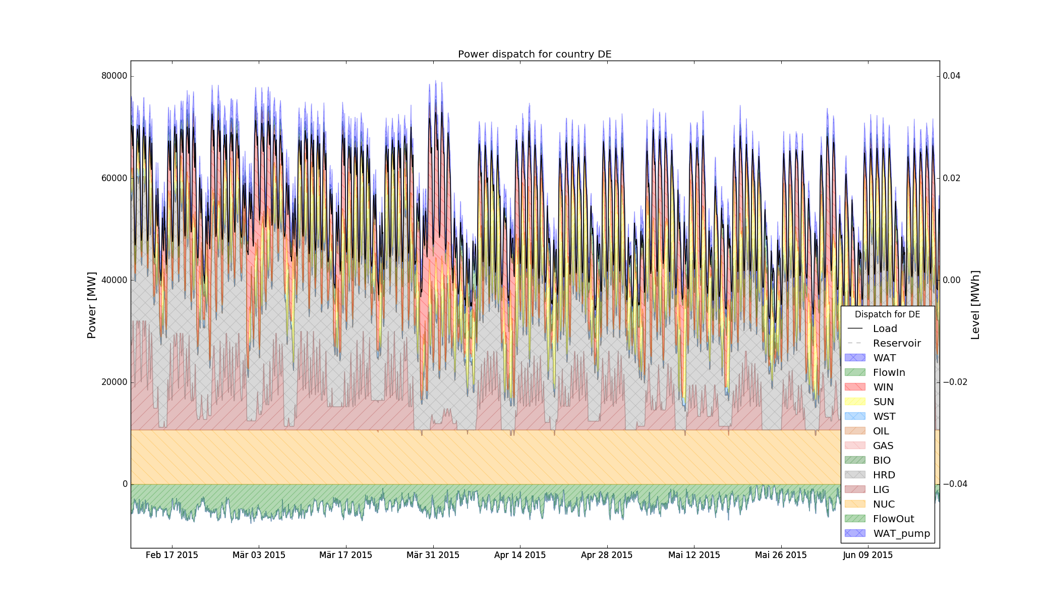
The power dispatch can be plotted for each simulated zone. In this plot, the units are aggregated by fuel type. The power consumed by storage units and the exportations are indicated as negative values.
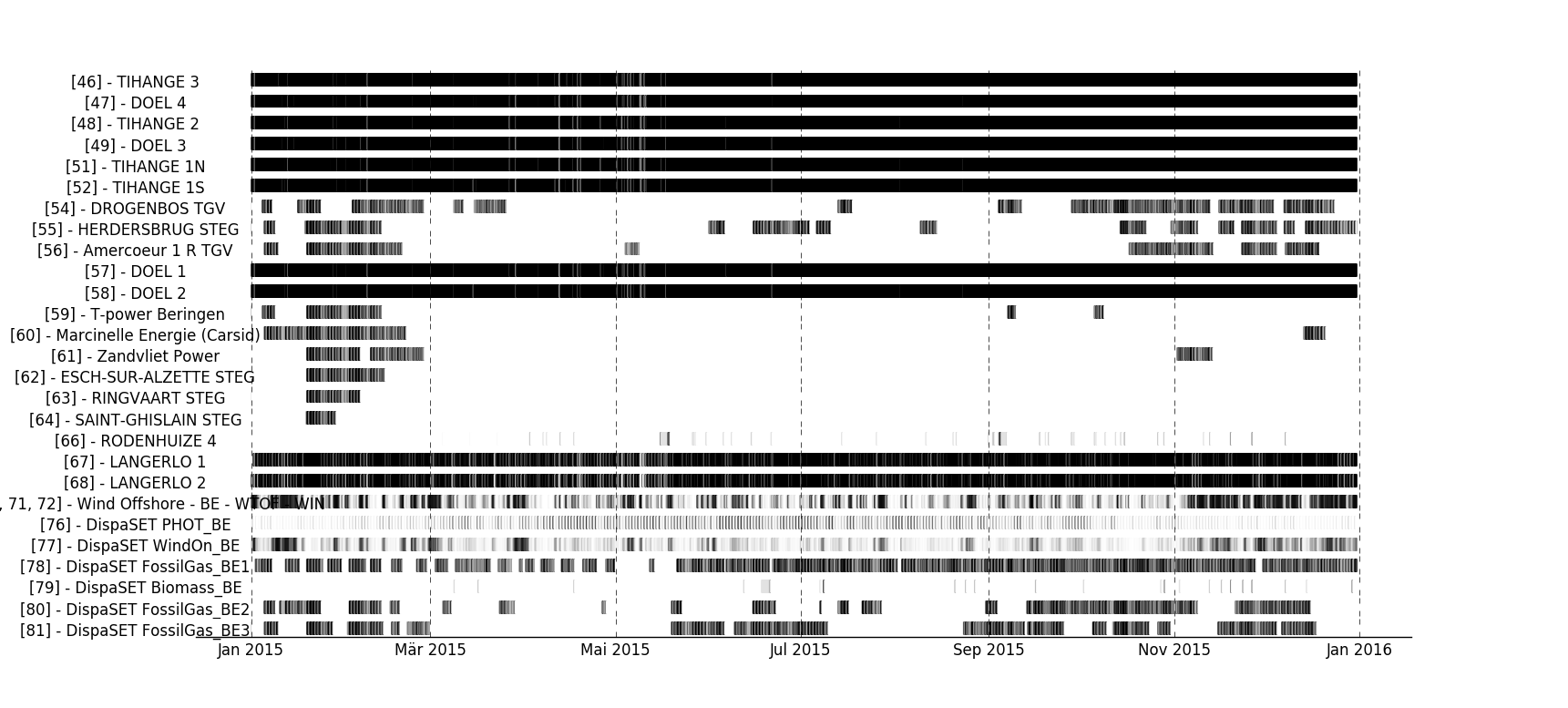
It is also interesting to display the results at the unit level to gain deeper insights regarding the dispatch. In that case, a plot is generated, showing the commitment status of all units in a zone at each timestep. Both the dispatch plot and the commitment plot can be called using the CountryPlots function.
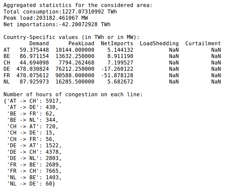
Some aggregated statistics on the simulations results can also be obtained, including the number of hours of congestion in each interconnection line, the yearly energy balances for each zone, the amount of lost load, etc.
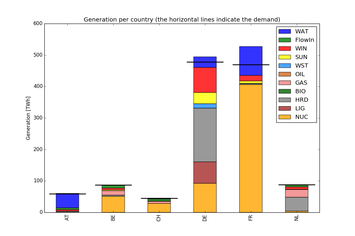
The yearly energy balance per fuel or per technology is also useful to compare the energy mix in each zone. This can be plotted using the EnergyBarPlot function, with the following results: