Model Description

The model is expressed as a MILP or LP problem. Continuous variables include the individual unit dispatched power, the shedded load and the curtailed power generation. The binary variables are the commitment status of each unit. The main model features can be summarized as follows:

Variables

Sets

Name	Description
au	All units
f	Fuel types
h	Hours
i(h)	Time step in the current optimization horizon
l	Transmission lines between nodes
mk	{DA: Day-Ahead, 2U: Reserve up, 2D: Reserve Down, flex}
n	Zones within each country (currently one zone, or node, per country)
nth	District heating zones (Multiple units can supply heat)
p	Pollutants
p2h(au)	Power to heat units
p2h2(s)	Power to H2 storage units
t	Power generation technologies
th(au)	Units with thermal storage
hu(au)	Heat only units
tr(t)	Renewable power generation technologies
u(au)	Generation units (all units minus P2HT units)
s(u)	Storage units (including hydro reservoirs)
chp(u)	CHP units
wat(s)	Hydro storage technologies
z(h)	Subset of every simulated hour

Parameters

Name	Units	Description
AvailabilityFactor(au,h)	%	Percentage of nominal capacity available
CHPPowerLossFactor(u)	%	Power loss when generating heat
CHPPowerToHeat(u)	%	Nominal power-to-heat factor
CHPMaxHeat(chp)	MW	Maximum heat capacity of chp plant
CHPType	n.a.	CHP Type
CommittedInitial(u)	n.a.	Initial commitment status
CostFixed(u)	EUR/h	Fixed costs
CostLoadShedding(n,h)	EUR/MWh	Shedding costs
CostRampDown(u)	EUR/MW	Ramp-down costs
CostRampUp(u)	EUR/MW	Ramp-up costs
CostShutDown(u)	EUR/u	Shut-down costs for one unit
CostStartUp(u)	EUR/u	Start-up costs for one unit
CostVariable(au,h)	EUR/MWh	Variable costs
CostHeatSlack(nth,h)	EUR/MWh	Cost of supplying heat via other means
CostH2Slack(p2h2,h)	EUR/MWh	Cost of supplying H2 by other means
Curtailment(n)	n.a.	Curtailment {binary: 1 allowed}
Demand(mk,n,h)	MW	Hourly demand in each zone
Efficiency(p2h,h)	%	Power plant efficiency
EmissionMaximum(n,p)	tP	Emission limit per zone for pollutant p
EmissionRate(u,p)	tP/MWh	Emission rate of pollutant p from unit u
FlowMaximum(l,h)	MW	Maximum flow in line
FlowMinimum(l,h)	MW	Minimum flow in line
Fuel(u,f)	n.a.	Fuel type used by unit u {binary: 1 u uses f}
HeatDemand(nth,h)	MWh/u	Heat demand profile for chp units
K_QuickStart(n)	n.a.	Part of the reserve that can be provided by offline quickstart units
LineNode(l,n)	n.a.	Line-zone incidence matrix {-1,+1}
LoadMaximum(au,h)	%	Maximum load given AF and OF
LoadShedding(n,h)	MW	Load that may be shed per zone in 1 hour
Location(au,n)	n.a.	Location {binary: 1 u located in n}
LocationTH(au,nth)	n.a.	Location {binary: 1 u located in nth)
LPFormulation	n.a.	Defines the equation that will be present: 1 for LP and 0 for MIP
Markup	EUR/MW	Markup
MTS	n.a.	Defines the equation that will be present: 1 for MidTermScheduling, 0 for normal optimization
Nunits(u)	n.a.	Number of units inside the cluster
OutageFactor(au,h)	%	Outage factor (100 % = full outage) per hour
PartLoadMin(u)	%	Percentage of minimum nominal capacity
PowerCapacity(au)	MW/u	Installed capacity
PowerInitial(u)	MW/u	Power output before initial period
PowerMinStable(au)	MW/u	Minimum power for stable generation
PowerMustRun(u)	MW	Minimum power output
PriceTransmission(l,h)	EUR/MWh	Price of transmission between zones
QuickStartPower(u,h)	MW/h/u	Available max capacity for tertiary reserve
RampDownMaximum(u)	MW/h/u	Ramp down limit
RampShutDownMaximum(u,h)	MW/h/u	Shut-down ramp limit
RampStartUpMaximum(u,h)	MW/h/u	Start-up ramp limit
RampUpMaximum(u)	MW/h/u	Ramp up limit
Reserve(t)	n.a.	Reserve provider {binary}
StorageCapacity(au)	MWh/u	Storage capacity (reservoirs)
StorageChargingCapacity(au)	MW/u	Maximum charging capacity
StorageChargingEfficiency(au)	%	Charging efficiency
StorageDischargeEfficiency(au)	%	Discharge efficiency
StorageInflow(u,h)	MWh/u	Storage inflows
StorageInitial(au)	MWh	Storage level before initial period
StorageMinimum(au)	MWh/u	Minimum storage level
StorageOutflow(u,h)	MWh/u	Storage outflows (spills)
StorageProfile(u,h)	%	Storage long-term level profile
StorageSelfDischarge(au)	%/day	Self discharge of the storage units
Technology(au,t)	n.a.	Technology type {binary: 1: u belongs to t}
TimeDownMinimum(u)	h	Minimum down time
TimeStep	h	Duration of a timestep of optimization
TimeUpMinimum(u)	h	Minimum up time
VOLL()	EUR/MWh	Value of lost load

NB: When the parameter is expressed per unit (“/u”), its value must be provided for one single unit (even in the case of a clustered formulation).

Optimization Variables

Name	Units	Description
AccumulatedOverSupply(n,h)	MWh	Accumulated oversupply due to the flexible demand
Committed(u,h)	n.a.	Unit committed at hour h {1,0}
CostStartUpH(u,h)	EUR	Cost of starting up
CostShutDownH(u,h)	EUR	Cost of shutting down
CostRampUpH(u,h)	EUR	Ramping cost
CostRampDownH(u,h)	EUR	Ramping cost
CurtailedPower(n,h)	MW	Curtailed power at node n
CurtailedHeat(n_th,h)	MW	Curtailed heat at node nth
Flow(l,h)	MW	Flow through lines
H2Output(au,h)	MWh	H2 output from H2 storage to fulfill the demand
Heat(au,h)	MW	Heat output by chp plant
HeatSlack(nth,h)	MW	Heat satisfied by other sources
Power(u,h)	MW	Power output
PowerConsumption(p2h,h)	MW	Power consumption by P2H
PowerMaximum(u,h)	MW	Power output
PowerMinimum(u,h)	MW	Power output
PtLDemand(au,h)	MW	Demand of H2 for PtL at each time step for P2HT units
Reserve_2U(u,h)	MW	Spinning reserve up
Reserve_2D(u,h)	MW	Spinning reserve down
Reserve_3U(u,h)	MW	Non spinning quick start reserve up
ShedLoad(n,h)	MW	Shed load
StorageInput(au,h)	MWh	Charging input for storage units
StorageLevel(au,h)	MWh	Storage level of charge
StorageSlack(au,h)	MWh	Unsatisfied storage level
Spillage(s,h)	MWh	Spillage from water reservoirs
SystemCost(h)	EUR	Total system cost
LL_MaxPower(n,h)	MW	Deficit in terms of maximum power
LL_RampUp(u,h)	MW	Deficit in terms of ramping up for each plant
LL_RampDown(u,h)	MW	Deficit in terms of ramping down
LL_MinPower(n,h)	MW	Power exceeding the demand
LL_2U(n,h)	MW	Deficit in reserve up
LL_3U(n,h)	MW	Deficit in reserve up - non spinning
LL_2D(n,h)	MW	Deficit in reserve down
WaterSlack(s)	MWh	Unsatisfied water level at end of optimization period

Free Variables

Name	Units	Description
SystemCostD	EUR	Total system cost for one optimization period
DemandModulation	MW	Difference between the flexible demand and the baseline

Integer Variables

Name	Units	Description
Committed(u,h)	n.a.	Number of unit committed at hour h {1 0} or integer
StartUp(u,h)	n.a.	Number of unit startups at hour h {1 0} or integer
ShutDown(u,h)	n.a.	Number of unit shutdowns at hour h {1 0} or integer

Optimisation model

The aim of this model is to represent with a high level of detail the short-term operation of large-scale power systems solving the so-called unit commitment problem. To that aim we consider that the system is managed by a central operator with full information on the technical and economic data of the generation units, the demands in each node, and the transmission network.

The unit commitment problem considered in this report is a simplified instance of the problem faced by the operator in charge of clearing the competitive bids of the participants into a wholesale day-ahead power market. In the present formulation the demand side is an aggregated input for each node, while the transmission network is modelled as a transport problem between the nodes (that is, the problem is network-constrained but the model does not include the calculation of the optimal power flows).

The unit commitment problem consists of two parts: i) scheduling the start-up, operation, and shut down of the available generation units, and ii) allocating (for each period of the simulation horizon of the model) the total power demand among the available generation units in such a way that the overall power system costs is minimized. The first part of the problem, the unit scheduling during several periods of time, requires the use of binary variables in order to represent the start-up and shut down decisions, as well as the consideration of constraints linking the commitment status of the units in different periods. The second part of the problem is the so-called economic dispatch problem, which determines the continuous output of each and every generation unit in the system. Therefore, given all the features of the problem mentioned above, it can be naturally formulated as a mixed-integer linear program (MILP). However, the problem can also be relaxed to a linear program (LP).

There is a possibility of Mid Term scheduling. It allows to optimize the level of energy in the storage reservoirs over a year and use it as endogeneous input in the optimization of interest. In that case, the equations linked to unit commitment are ignored.

Since our goal is to model a large European interconnected power system, we have implemented a so-called tight and compact formulation, in order to simultaneously reduce the region where the solver searches for the solution and increase the speed at which the solver carries out that search. Tightness refers to the distance between the relaxed and integer solutions of the MILP and therefore defines the search space to be explored by the solver, while compactness is related to the amount of data to be processed by the solver and thus determines the speed at which the solver searches for the optimum. Usually tightness is increased by adding new constraints, but that also increases the size of the problem (decreases compactness), so both goals contradict each other and a trade-off must be found.

Objective function

The goal of the unit commitment problem is to minimize the total power system costs (expressed in EUR in equation ), which are defined as the sum of different cost items, namely: start-up and shut-down, fixed, variable, ramping, transmission-related and load shedding (voluntary and involuntary) costs.

\[\begin{split}\begin{split} min & \Big[ \sum_{u,i} CostFixed_{u} \cdot Committed_{u,i} \cdot TimeStep \\ & + \sum_{u,i} ( CostStartUpH_{u,i} + CostShutDownH_{u,i}) \\ & + \sum_{u,i} (CostRampUpH_{u,i} + CostRampDownH_{u,i}) \\ & + \sum_{u,i} CostVariable_{u,i} \cdot Power_{u,i} \cdot TimeStep \\ & + \sum_{hu,i} CostVariable_{hu,i} \cdot Heat_{hu,i} \cdot TimeStep \\ & + \sum_{l,i} PriceTransimission_{l,i} \cdot Flow_{l,i} \cdot TimeStep \\ & + \sum_{n,i} CostLoadShedding_{i,n} \cdot ShedLoad_{i,n} \cdot TimeStep \\ & + \sum_{th,i} CostHeatSlack_{nth,i} \cdot HeatSlack_{nth,i} \cdot TimeStep) \\ & + \sum_{p2h2,i} CostH2Slack_{p2h2,i} \cdot StorageSlack_{p2h2,i} \cdot TimeStep \\ & + \sum_{chp,i} CostVariable_{chp,i} \cdot CHPPowerLossFactor_{chp} \cdot Heat_{chp,i} \cdot TimeStep) \\ & + \sum_{i,n} VOLL_{Power} \cdot \left( \mathit{LL}_{MaxPower,i,n} + \mathit{LL}_{MinPower,i,n} \right) \cdot TimeStep \\ & + \sum_{i,n} 0.8 \cdot VOLL_{Reserve} \cdot \left( LL_{2U,i,n} + LL_{2D,i,n}+ LL_{3U,i,n} \right) \cdot TimeStep \\ & + \sum_{u,i} 0.7 \cdot VOLL_{Ramp} \cdot \left( LL_{RampUp,u,i} + LL_{RampDown,u,i} \right)\cdot TimeStep \\ & + \sum_{s,i} CostOfSpillage \cdot spillage_{s,i} \\ & + \sum_{s,i} WaterValue\cdot WaterSlack_s \Big] \end{split}\end{split}\]

The costs can be broken down as:

• Fixed costs: depending on whether the unit is on or off.

• Variable costs: stemming from the power output of the units.

• Start-up costs: due to the start-up of a unit.

• Shut-down costs: due to the shut-down of a unit.

• Ramp-up: emerging from the ramping up of a unit.

• Ramp-down: emerging from the ramping down of a unit.

• Load shed: due to necessary load shedding.

• Transmission: depending of the flow transmitted through the lines.

• Loss of load: power exceeding the demand or not matching it, ramping and reserve.

• spillage: due to spillage in storage.

• H2: cost of unsatisfied hydrogen by production from electrolyzers

• Water : cost of water coming from unsatisfied water level at the end of the optimization period.

The variable production costs (in EUR/MWh), are determined by fuel and emission prices corrected by the efficiency (which is considered to be constant for all levels of output in this version of the model) and the emission rate of the unit (equation ):

\[\begin{split}\begin{align} \mathit{CostVariable}_{au,h}= &\mathit{Markup}_{au,h} + \sum _{n,f}\left(\frac{\mathit{Fuel}_{au,f} \cdot \mathit{FuelPrice}_{n,f,h} \cdot \mathit{Location}_{au,n}}{\mathit{Efficiency}_u}\right)\\ & + \sum _p\left(\mathit{EmissionRate}_{au,p} \cdot \mathit{PermitPrice}_p\right) \end{align}\end{split}\]

The variable cost includes an additional mark-up parameter that can be used for calibration and validation purposes.

From version 2.3, Dispa-SET uses a 3 integers formulations of the up/down status of all units. According to this formulation, the number of start-ups and shut-downs is at each time step is computed by:

\[\mathit{Committed}_{u,i}-\mathit{Committed}_{u,i-1} = \mathit{StartUp}_{u,i} - \mathit{ShutDown}_{u,i}\]

The start-up and shut-down costs are positive variables, calculated from the number of startups/shutdowns at each time step:

\[\begin{split}\begin{align} \mathit{CostStartUp}_{u,i} &= \mathit{CostStartUp}_u \cdot \mathit{StartUp}_{u,i}\\ \mathit{CostShutDown}_{u,i} &= \mathit{CostShutDown}_u \cdot \mathit{ShutDown}_{u,i} \end{align}\end{split}\]

Renewable units are enforced commited when the availability factor is non null and the outage factor is not 1 and decommited in the other case.

Ramping costs are defined as positive variables (i.e. negative costs are not allowed) and are computed with the following equations:

\[\begin{split}\begin{align} \mathit{CostRampUp}_{u,i} &\geq \mathit{CostRampUp}_u \cdot \left(\mathit{Power}_{u,i}-\mathit{Power}_{u,i-1}\right)\\ \mathit{CostRampDown}_{u,i} &\geq \mathit{CostRampDown}_u \cdot (\mathit{Power}_{u,i-1}-\mathit{Power}_{u,i}) \end{align}\end{split}\]

It should be noted that in case of start-up and shut-down, the ramping costs are added to the objective function. Using start-up, shut-down and ramping costs at the same time should therefore be performed with care.

In the current formulation, all other costs (fixed and variable costs, transmission costs, load shedding costs) are considered as exogenous parameters.

As regards load shedding, the model considers the possibility of voluntary load shedding resulting from contractual arrangements between generators and consumers. Additionally, in order to facilitate tracking and debugging of errors, the model also considers some variables representing the capacity the system is not able to provide when the minimum/maximum power, reserve, or ramping constraints are reached. These lost loads are a very expensive last resort of the system used when there is no other choice available. The different lost loads are assigned very high values (with respect to any other costs). This allows running the simulation without infeasibilities, thus helping to detect the origin of the loss of load. In a normal run of the model, without errors, all these variables are expected to be equal to zero.

Day-ahead energy balance

The main constraint to be met is the supply-demand balance, for each period and each zone, in the day-ahead market (equation ). According to this restriction, the sum of all the power produced by all the units present in the node (including the power generated by the storage units), the power injected from neighbouring nodes, and the curtailed power from intermittent sources is equal to the load in that node, plus the power consumed for energy storage, minus the load interrupted and the load shed.

\[\begin{split}\begin{align} \sum _u\left(\mathit{Power}_{u,i} \cdot \mathit{Location}_{u,n}\right) + \sum _l\left(\mathit{Flow}_{l,i} \cdot \mathit{LineNode}_{l,n}\right)\\ = \mathit{Demand}_{\mathit{DA},n,h} + \sum _s\left(\mathit{StorageInput}_{s,h} \cdot \mathit{Location}_{s,n}\right) -\mathit{ShedLoad}_{n,i} \\ + \sum_{p2h} \mathit{PowerConsumption}_{p2h,i} \cdot \mathit{Location}_{p2h,n} - \mathit{LL_{MaxPower}}_{n,i} + \mathit{LL_{MinPower}}_{n,i} \end{align}\end{split}\]

Reserve constraints

Besides the production/demand balance, the reserve requirements (upwards and downwards) in each node must be met as well. In Dispa-SET, three types of reserve requirements are taken into account:

• Upward secondary reserve (2U): reserve that can only be covered by spinning units

• Downward secondary reserve (2D): reserve that can only be covered by spinning units

• Upward tertiary reserve (3U): reserve that can be covered either by spinning units or by quick-start offline units

The secondary reserve capability of committed units is limited by the capacity margin between current and maximum power output:

\[\begin{split}\begin{align} \mathit{Reserve_{2U}}_{u,i} \leq& \mathit{PowerCapacity}_u \cdot \mathit{AvailabilityFactor}_{u,i} \cdot (1-\mathit{OutageFactor}_{u,i}) \cdot \mathit{Committed}_{u,i}\\ & - \mathit{Power}_{u,i} \end{align}\end{split}\]

The same applies to the downwards secondary reserve capability, with an additional term to take into account the downard reserve capability of storage units:

\[\begin{split}\begin{align} \mathit{Reserve_{2D}}_{u,i} \leq &\; \mathit{Power}_{u,i} - \mathit{PowerMustRun}_{u,i} \cdot \mathit{Committed}_{u,i} \\ &+ (\mathit{StorageChargingCapacity}_u \cdot \mathit{Nunits}_u - \mathit{StorageInput}_{u,i}) \end{align}\end{split}\]

The quick start (non-spining) reserve capability is given by:

\[\mathit{Reserve_{3U}}_{u,i} \leq (\mathit{Nunits}_u - \mathit{Committed}_{u,i}) \cdot \mathit{QuickStartPower}_{u,i} \cdot \mathit{TimeStep}\]

The secondary reserve demand should be fulfilled at all times by all the plants allowed to participate in the reserve market:

\[\begin{split}\begin{align} \mathit{Demand}_{2U,n,h} \leq & \sum _{u,t}\left(\mathit{Reserve_{2U}}_{u,i} \cdot \mathit{Technology}_{u,t} \cdot \mathit{Reserve}_t \cdot \mathit{Locatio}n_{u,n}\right)\\ & + \mathit{LL_{2U}}_{n,i} \end{align}\end{split}\]

The same equation applies to downward reserve requirements (2D).

The tertiary reserve can also be provided by non-spinning units. The inequality is thus transformed into:

\[\begin{split}\begin{align} \mathit{Demand}_{3U,n,h} \leq & \sum _{u,t}[(\mathit{Reserve_{2U}}_{u,i} + \mathit{Reserve_{3U}}_{u,i} ) \cdot \mathit{Technology}_{u,t} \cdot \mathit{Reserve}_t \cdot \mathit{Locatio}n_{u,n} ]\\ &+ \mathit{LL_{3U}}_{n,i} \end{align}\end{split}\]

Reserve Requirements

The reserve requirements are defined by the users. In case no input is provided, one among the three methods modeled in Dispa-SET and briefly described here can be selected.

The first method proposed to evaluate the needs for reserves is static and based on an empirical formula which is function of the maximum expected load for each day. The empirical formula is described by:

\[\mathit{Demand}_{2U,n,i}=\sqrt{10 \cdot \underset h{\mathit{max}}\left(\mathit{Demand}_{\mathit{DA},n,h}\right) + 150^2}-150\]

Downward reserves are defined as 50% of the upward margin:

\[\mathit{Demand}_{2D,n,h}=0.5 \cdot \mathit{Demand}_{2U,n,h}\]

The second formulation proposed by Dispa-SET is dynamic and based on the (3+5)% rule. Reserve requirements are computed as a fraction of the forecasted demand and available wind and solar power at a certain hour of the day. Here the formula:

\[\begin{split}\begin{align} \mathit{Demand}_{2U,n,h}=0.03 \cdot \mathit{Demand}_{\mathit{DA},n,h} \\ + 0.05 \cdot \mathit{AvailableWindPower}_{u,i} + 0.05 \cdot \mathit{AvailablePhotPower}_{u,i} \end{align}\end{split}\]

In this case downward reserves are equal to upward reserves.

The third and last method proposed in Dispa-SET is dynamic and probabilistic. It accounts for reserve requirements as the sum of two components as follows:

\[\begin{split}\begin{align} \mathit{Demand}_{2U,n,h}= \sqrt{10 \cdot \mathit{Demand}_{\mathit{DA},n,h} + 150^2}-150 \\ + 2.74 \cdot \sqrt{ \sigma_{L,n,h}^2 + \sigma_{W,n,h}^2 + \sigma_{S,n,h}^2} \end{align}\end{split}\]

where the second part of the function exploits the standard deviations of demand, solar and wind power forecast error functions assuming a confidence level equal to 99.7%. Also in this last case downward reserves are equal to upward reserves.

Power output bounds

The minimum power output is determined by the must-run or stable generation level of the unit if it is committed:

\[\mathit{Power}\mathit{MustRun}_{u,i} \cdot \mathit{Committed}_{u,i} \leq \mathit{Power}_{u,i}\]

In the particular case of CHP unit (extration type or power-to-heat type), the minimum power is defined for for a heat demand equal to zero. If the unit produces heat, the minimum power must be reduced according to the power loss factor and the previous equation is replaced by:

\[ \begin{align}\begin{aligned}\mathit{Power}\mathit{MustRun}_{chp,i} \cdot \mathit{Committed}_{chp,i}\\- \mathit{StorageInput}_{chp,i} \cdot \mathit{CHPPowerLossFactor}_u\\ \leq \mathit{Power}_{chp,i}\end{aligned}\end{align} \]

The power output is limited by the available capacity, if the unit is committed:

\[ \begin{align}\begin{aligned}\mathit{Power}_{u,i}\\ \leq \mathit{PowerCapacity}_u \cdot \mathit{AvailabilityFactor}_{u,i} \cdot (1-\mathit{OutageFactor}_{u,i}) \cdot \mathit{Committed}_{u,i}\end{aligned}\end{align} \]

The availability factor is used for renewable technologies to set the maximum time-dependent generation level. It is set to one for the traditional power plants. The outage factor accounts for the share of unavailable power due to planned or unplanned outages.

Ramping Constraints

Each unit is characterized by a maximum ramp up and ramp down capability. This is translated into the following inequality for the case of ramping up:

\[ \begin{align}\begin{aligned}\mathit{Power}_{u,i} - \mathit{Power}_{u,i-1} \leq\\(\mathit{Committed}_{u,i} - \mathit{StartUp}_{u,i}) \cdot \mathit{RampUpMaximum}_{u} \cdot \mathit{TimeStep}\\+ \mathit{StartUp}_{u,i} \cdot \mathit{RampStartUpMaximum}_{u} \cdot \mathit{TimeStep}\\- \mathit{ShutDown}_{u,i} \cdot \mathit{PowerMustRun}_{u,i}\\+ \mathit{LL_{RampUp}}_{u,i}\end{aligned}\end{align} \]

and for the case of ramping down:

\[ \begin{align}\begin{aligned}\mathit{Power}_{u,i-1} - \mathit{Power}_{u,i} \leq\\(\mathit{Committed}_{u,i} - \mathit{ShutDown}_{u,i}) \cdot \mathit{RampDownMaximum}_{u} \cdot \mathit{TimeStep}\\+ \mathit{ShutDown}_{u,i} \cdot \mathit{RampShutDownMaximum}_{u} \cdot \mathit{TimeStep}\\- \mathit{StartUp}_{u,i} \cdot \mathit{PowerMustRun}_{u,i}\\+ \mathit{LL_{RampDown}}_{u,i}\end{aligned}\end{align} \]

Note that this formulation is valid for both the clustered formulation and the binary formulation. In the latter case (there is only one unit u), if the unit remains committed, the inequality simplifies into:

\[ \begin{align}\begin{aligned}\mathit{Power}_{u,i} - \mathit{Power}_{u,i-1} \leq\\\mathit{RampUpMaximum}_{u} \cdot \mathit{TimeStep} + \mathit{LL_{RampUp}}_{u,i}\end{aligned}\end{align} \]

If the unit has just been committed, the inequality becomes:

\[ \begin{align}\begin{aligned}\mathit{Power}_{u,i} - \mathit{Power}_{u,i-1} \leq\\\mathit{RampStartUpMaximum}_{u} \cdot \mathit{TimeStep} + \mathit{LL_{RampUp}}_{u,i}\end{aligned}\end{align} \]

And if the unit has just been stopped:

\[ \begin{align}\begin{aligned}\mathit{Power}_{u,i} - \mathit{Power}_{u,i-1} \leq\\- \mathit{PowerMustRun}_{u,i} + \mathit{LL_{RampUp}}_{u,i}\end{aligned}\end{align} \]

Minimum up and down times

The operation of the generation units is also limited as well by the amount of time the unit has been running or stopped. In order to avoid excessive ageing of the generators, or because of their physical characteristics, once a unit is started up, it cannot be shut down immediately. Reciprocally, if the unit is shut down it may not be started immediately.

To model this in MILP, the number of startups/shutdowns in the last N hours must be limited, N being the minimum up or down time. For the minimum up time, the number of startups during this period cannot be higher than the number of currently committed units:

\[\sum _{ii=i-\frac{\mathit{TimeUpMinimum}_u}{\mathit{TimeStep}}}^{i} \mathit{StartUp}_{u,ii} \leq \mathit{Committed}_{u,i}\]

i.e. the currently committed units are not allowed to have performed multiple on/off cycles between the optimization time minus TimeUpMinimum and the optimization time. The implied number of periods is computed by the ratio of TimeUpMinimum and TimeStep. If TimeUpMinimum is not a multiple of TimeStep, their fraction is rounded upwards. In case of a binary formulation (Nunits=1), if the unit is ON at time i, only one startup is allowed in the last TimeUpMinimum periods. If the unit is OFF at time i, no startup is allowed.

A similar inequality can be written for the ninimum down time:

\[\sum _{ii=i-\frac{\mathit{TimeDownMinimum}_u}{\mathit{TimeStep}}}^{i} \mathit{ShutDown}_{u,ii} \leq \mathit{Nunits}_u - \mathit{Committed}_{u,i}\]

Storage-related constraints

Generation units with energy storage capabilities (large hydro reservoirs, pumped hydro storage units, hydrogen storage units or batteries) must meet additional restrictions related to the amount of energy stored. Storage units are considered to be subject to the same constraints as non-storage power plants. In addition to those constraints, storage-specific restrictions are added for the set of storage units (i.e. a subset of all units). These restrictions include the storage capacity, inflow, outflow, charging, charging capacity, charge/discharge efficiencies, etc. Discharging is considered as the standard operation mode and is therefore linked to the Power variable, common to all units.

The first constraint imposes that the energy stored by a given unit is bounded by a minimum value:

\[\mathit{StorageMinimum}_s \leq \mathit{StorageLevel}_{s,i} \cdot \mathit{Nunits}_s\]

In the case of a storage unit, the availability factor applies to the charging/discharging power, but also to the storage capacity. The storage level is thus limited by:

\[\mathit{StorageLevel}_{s,i} \leq \mathit{StorageCapacity}_s \cdot \mathit{AvailabilityFactor}_{s,i} \cdot \mathit{Nunits}_s\]

The energy added to the storage unit is limited by the charging capacity. Charging is allowed only if the unit is not producing (discharging) at the same time (i.e. if Committed, corresponding to the normal mode, is equal to 0).

\[ \begin{align}\begin{aligned}\mathit{StorageInput}_{s,i} \leq\\\mathit{StorageChargingCapacity}_s \cdot (\mathit{Nunits}_s-\mathit{Committed}_{s,i})\end{aligned}\end{align} \]

Discharge is limited by the level of charge of the storage unit:

\[ \begin{align}\begin{aligned}\frac{\mathit{Power}_{i,s}\cdot \mathit{TimeStep}}{\mathit{StorageDischargeEfficienc}y_s} + \mathit{StorageOutflow}_{s,i} \cdot \mathit{Nunits}_s \cdot \mathit{TimeStep}\\+ \mathit{Spillage}_{wat,i} -\mathit{StorageInflow}_{s,i} \cdot \mathit{Nunits}_s \cdot \mathit{TimeStep} - StorageSlack_{p2h2,i}\\\leq \mathit{StorageLevel}_{s,i}\end{aligned}\end{align} \]

It is worthwhile to note that StorageInflow and StorageOuflow must be multiplied by the number of units because they are defined for a single storage plant. On the contrary StorageLevel, Spillage and Power are defined for all units s. StorageInflow and Storage Outflow are predefined time series, whose meaning depends on the type of storage units: for hydro units, it is the natural water flows. For hydrogen units, StorageInflow is 0 at all times, but StorageOutflow represents the hydrogen demand (for fuel cell vehicles, industries,…). For batteries, both parameters are null at all times.

Charge is limited by the level of charge of the storage unit:

\[ \begin{align}\begin{aligned}\mathit{StorageInput}_{s,i} \cdot \mathit{StorageChargingEfficiency}_s \cdot \mathit{TimeStep}\\- \mathit{StorageOutflow}_{s,i} \cdot \mathit{Nunits}_s \cdot \mathit{TimeStep}- \mathit{Spillage}_{wat,i}\\+ \mathit{StorageInflow}_{s,i} \cdot \mathit{Nunits}_s \cdot \mathit{TimeStep} + StorageSlack_{p2h2,i}\\\leq \mathit{StorageCapacity}_s \cdot \mathit{AvailabilityFactor}_{s,i}\\- \mathit{StorageLevel}_{s,i}\end{aligned}\end{align} \]

Besides, the energy stored in a given period is given by the energy stored in the previous period, net of charges and discharges:

\[ \begin{align}\begin{aligned}\mathit{StorageLevel}_{s,i-1} + \mathit{StorageInflow}_{s,i} \cdot \mathit{Nunits}_s \cdot \mathit{TimeStep}\\+ \mathit{StorageInput}_{s,i} \cdot \mathit{StorageChargingEfficiency}_s \cdot \mathit{TimeStep} + StorageSlack_{p2h2,i}\\= \mathit{StorageLevel}_{s,i} + \mathit{StorageOutflow}_{s,i} \cdot \mathit{Nunits}_s \cdot \mathit{TimeStep}\\+ Spillage_{wat,i} + \frac{\mathit{Power}_{s,i}\cdot \mathit{TimeStep}}{\mathit{StorageDischargeEfficienc}y_s}\end{aligned}\end{align} \]

Some storage units are equiped with large reservoirs, whose capacity at full load might be longer than the optimisation horizon. Therefore, a minimum level constraint is required for the last hour of the optimisation, which otherwise would systematically tend to empty the reservoir as much a possible. An exogenous minimum profile is thus provided and the following constraint is applied:

\[\mathit{StorageLevel}_{s,N} \geq StorageFinalMin_{s} + WaterSlack_{wat}\]

where N is the last period of the optimization horizon, StorageProfile is a non-dimensional minimum storage level provided as an exogenous input and WaterSlack is a variable defining the unsatified water level. The price associated to that water is very high.

Heat balance

In Dispa-SET heat demand is specified for individual heating zones (nth). It can be covered either by a CHP plant, P2HT unit or by alternative heat supply options (Heat Slack) or a combination of all three types of units.

\[\begin{split}\sum _{chp} Heat_{chp,i} \cdot LocationTH_{chp,nth} \\ + \sum _{p2h} (Heat_{p2h,i} \cdot LocationTH_{p2h, nth}) \\ + \sum _{hu} (Heat_{hu,i} \cdot LocationTH_{hu, nth}) \\ = HeatDemand_{nth,i} - HeatSlack_{nth,i}\end{split}\]

Heat output cosntraints

Simmilarly to Power output constraints, Heat output must be below maximum generation capacity.

\[Heat_{hu,i} \leq PowerCapacity_{hu} \cdot \mathit{AvailabilityFactor}_{hu,i} \cdot (1-\mathit{OutageFactor}_{hu,i})\]

Heat production constraints (CHP plants only)

In DispaSET Power plants can be indicated as CHP which gives them the possibility to satisfy heat demand.

The following heat balance constraints are used for any CHP and P2H plant types.

\[StorageInput_{chp,i} \leq CHPMaxHeat_{chp} \cdot \mathit{Nunits}_{chp}\]

The constraints between heat and power production differ for each plant design and are explained within the following subsections.

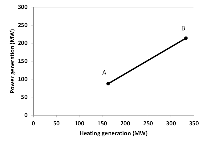
Steam plants with Backpressure turbine

This options includes steam-turbine based power plants with a backpressure turbine. The feasible operating region is between AB. The slope of the line is the heat to power ratio.

\[Power_{chp,i} = StorageInput_{chp,i} \cdot CHPPowerToHeat_{chp}\]

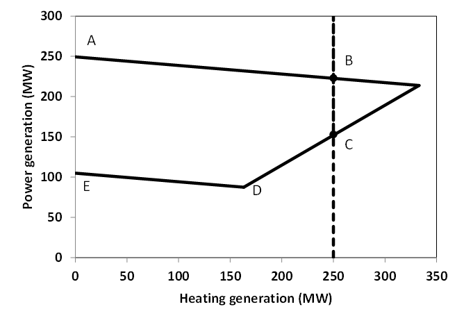
Steam plants with Extraction/condensing turbine

This options includes steam-turbine based power plants with an extraction/condensing turbine. The feasible operating region is within ABCDE. The vertical dotted line BC corresponds to the minimum condensation line (as defined by CHPMaxHeat). The slope of the DC line is the heat to power ratio and the slope of the AB line is the inverse of the power penalty ratio.

\[Power_{chp,i} \geq StorageInput_{chp,i} \cdot CHPPowerToHeat_{chp}\]

\[ \begin{align}\begin{aligned}Power_{chp,i} \leq PowerCapacity_{chp} \cdot \mathit{Nunits} -\\StorageInput_{chp,i} \cdot CHPPowerLossFactor_{chp}\end{aligned}\end{align} \]

\[Power_{chp,i} \geq PowerMustRun_{chp,i} - StorageInput_{chp,i} \cdot CHPPowerLossFactor_{chp}\]

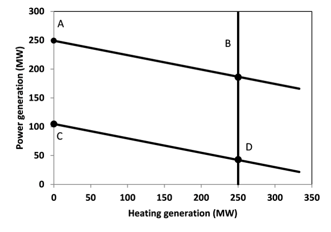
Power plant coupled with any power to heat option

This option includes power plants coupled with resistance heater or heat pumps. The feasible operating region is between ABCD. The slope of the AB and CD line is the inverse of the COP or efficiency. The vertical dotted line corresponds to the heat pump (or resistance heater) thermal capacity (as defined by CHPMaxHeat)

\[Power_{chp,i} \leq PowerCapacity_{chp} - StorageInput_{chp,i} \cdot CHPPowerLossFactor_{chp}\]

\[Power_{chp,i} \geq PowerMustRun_{chp,i} - StorageInput_{chp,i} \cdot CHPPowerLossFactor_{chp}\]

Power to heat units (labeled as P2HT technology)

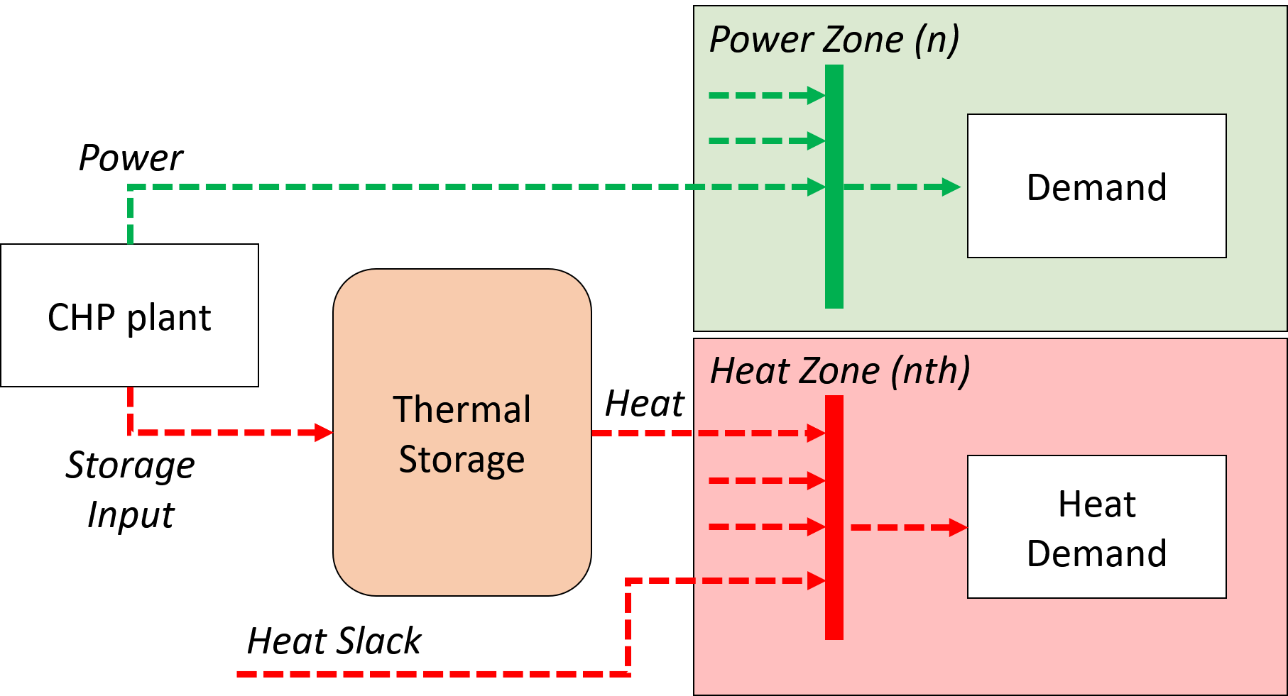
Oposite to power plants coupled with any power to heat option, individual power to heat units (technology = P2HT) have only one mode of operation. They consume power to generate heat. In Dispa-SET these units are either small scale residential heat pumps or electric heaters or large industrial or district heating devices power by electricity. A shematic overview of these units is shown below:

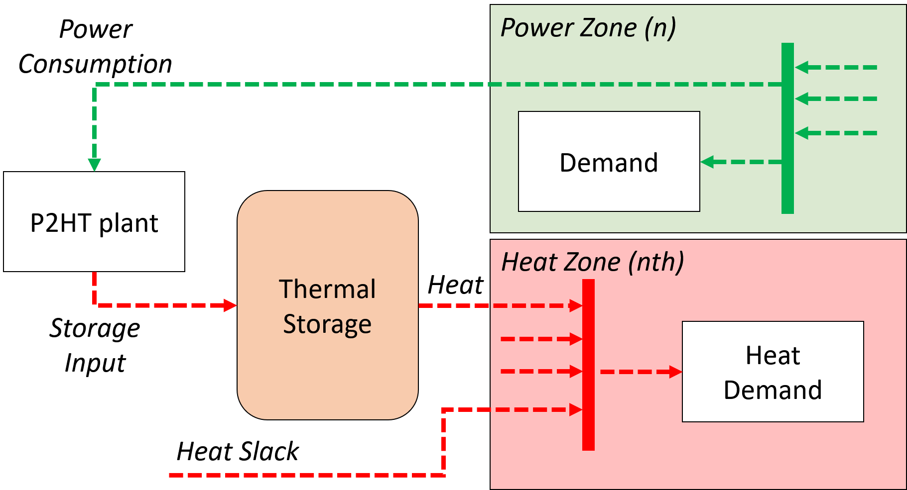
They are subjet to the following set of constraints:

\[StorageInput_{p2h,i} = PowerConsumption_{p2h,i} \cdot Efficiency_{p2h,i}\]

\[PowerConsumption_{p2h,i} \leq PowerCapacity_{p2h} \cdot Nunits_{p2h}\]

Heat Storage

Heat storage is modeled in a similar way as electric storage as follows:

Heat Storage balance:

\[ \begin{align}\begin{aligned}StorageLevel_{th,i-1} +StorageInput_{th,i} \cdot TimeStep =\\StorageLevel_{th,i} +Heat_{th,i} \cdot TimeStep\\ + StorageSelfDischarge_{th} \cdot StorageLevel_{th,i}\cdot TimeStep/24\end{aligned}\end{align} \]

Storage level must be above a minimum and below storage capacity:

\[StorageMinimum_{th} \cdot Nunits_{th} \leq StorageLevel_{chp,i} \leq StorageCapacity_{th} \cdot \mathit{Nunits}_{th}\]

Emission limits

The operating schedule also needs to take into account any cap on the emissions (not only CO2) from the generation units existing in each node:

\[ \begin{align}\begin{aligned}\sum _u\left(\mathit{Power}_{u,i} \cdot \mathit{EmisionRate}_{u,p} \cdot TimeStep \cdot \mathit{Location}_{u,n}\right)\\\leq \mathit{EmisionMaximum}_{n,p}\end{aligned}\end{align} \]

It is important to note that the emission cap is applied to each optimisation horizon: if a rolling horizon of one day is adopted for the simulation, the cap will be applied to all days instead of the whole year.

Network-related constraints

The flow of power between nodes is limited by the capacities of the transmission lines:

\[ \begin{align}\begin{aligned}\mathit{FlowMinimum}_{l,i} \leq \mathit{Flow}_{l,i}\\\mathit{Flow}_{l,i} \leq \mathit{FlowMaximum}_{l,i}\end{aligned}\end{align} \]

In this model a simple Net Transfer Capacity (NTC) between countries approach is followed. No DC power flow or Locational Marginal Pricing (LMP) model is implemented.

Load shedding

If load shedding is allowed in a node, the amount of shed load is limited by the shedding capacity contracted on that particular node (e.g. through interruptible industrial contracts)

\[\mathit{ShedLoad}_{n,i} \leq \mathit{LoadShedding}_{n,i}\]

Linear Program (LP) optimization

A possible simplification of the model is to run it as a LP instead of MILP. In that case, the LPFormulation parameter needs to be set to 1 (and to 0 otherwise).

In that case, the commitment status variables Commited, StartUp and ShutDown are not defined as binary and Commited is set smaller than 1. The equations describing the cost of starting up and shutting down are ignored, as well as the ones enforcing minimum up and down times.

Mid Term Scheduling (MTS)

As will be explained in more details hereunder, MTS allows to pre-define storage levels during the whole year based on a simplified equations.

Model in MTS mode

When MTS is activated, some equations are dropped/modified. MTS mode is activated by setting parameter MTS to 1. In this configuration, all equations concerning unit commitment are not considered and the binary variables Committed, StartUp and ShutDown are not defined. The following constraints are therefore ignored:

• The commitment equations

• The minimum Up and Down times equations

• The Ramp up and Ramp down limitation equations

Also, due to the absence of the variable Committed, some equations are modified. Firstly, the cost equation is modified as follow:

\[\begin{split}\begin{split} min & \Big[ \sum_{u,i} CostFixed_{u} \cdot TimeStep \\ & + \sum_{u,i} ( CostStartUpH_{u,i} + CostShutDownH_{u,i}) \\ & + \sum_{u,i} (CostRampUpH_{u,i} + CostRampDownH_{u,i}) \\ & + \sum_{u,i} CostVariable_{u,i} \cdot Power_{u,i} \cdot TimeStep \\ & + \sum_{hu,i} CostVariable_{hu,i} \cdot Heat_{hu,i} \cdot TimeStep \\ & + \sum_{l,i} PriceTransimission_{l,i} \cdot Flow_{l,i} \cdot TimeStep \\ & + \sum_{n,i} CostLoadShedding_{i,n} \cdot ShedLoad_{i,n} \cdot TimeStep \\ & + \sum_{th,i} CostHeatSlack_{th,i} \cdot HeatSlack_{th,i} \cdot TimeStep) \\ & + \sum_{p2h2,i} CostH2Slack_{p2h2,i} \cdot StorageSlack_{p2h2,i} \cdot TimeStep) \\ & + \sum _{chp,i} CostVariable_{chp,i} \cdot CHPPowerLossFactor_{chp} \cdot Heat_{chp,i} \cdot TimeStep) \\ & + \sum_{i,n} VOLL_{Power} \cdot \left( \mathit{LL}_{MaxPower,i,n} + \mathit{LL}_{MinPower,i,n} \right) \cdot TimeStep \\ & + \sum_{i,n} 0.8 \cdot VOLL_{Reserve} \cdot \left( LL_{2U,i,n} + LL_{2D,i,n}+ LL_{3U,i,n} \right) \cdot TimeStep \\ & + \sum_{s,i} CostOfSpillage \cdot spillage_{s,i} \\ & + \sum_{s,i} WaterValue\cdot WaterSlack_s \Big] \end{split}\end{split}\]

The upwards and downwards secondary reserve capabilities of units becomes:

\[\begin{split}\begin{align} \mathit{Reserve_{2U}}_{u,i} \leq& \mathit{PowerCapacity}_u \cdot \mathit{AvailabilityFactor}_{u,i} \cdot (1-\mathit{OutageFactor}_{u,i}) \\ & - \mathit{Power}_{u,i} \\ \mathit{Reserve_{2D}}_{u,i} \leq &\; \mathit{Power}_{u,i} + (\mathit{StorageChargingCapacity}_u \cdot \mathit{Nunits}_u - \mathit{StorageInput}_{u,i}) \end{align}\end{split}\]

Also the non spinning reserve is modified:

\[\mathit{Reserve_{3U}}_{u,i} \leq \mathit{Nunits}_u \cdot \mathit{QuickStartPower}_{u,i} \cdot \mathit{TimeStep}\]

The output power available for each unit is now expressed as:

\[\mathit{Power}_{u,i} \leq \mathit{PowerCapacity} \cdot \mathit{AvailibilityFactor} \cdot (1- \mathit{OutageFactor})\]

Finally, the maximum capacity of storage charging is:

\[\mathit{StorageInput}_{s,i} \leq \mathit{StorageChargingCapacity}_s \cdot \mathit{Nunits}_s\]

Rolling Horizon

The mathematical problem described in the previous sections could in principle be solved for a whole year split into time steps, but with all likelihood the problem would become extremely demanding in computational terms when attempting to solve the model with a realistically sized dataset. Therefore, the problem is split into smaller optimization problems that are run recursively throughout the year.

The following figure shows an example of such approach, in which the optimization horizon is two days, including a look-ahead (or overlap) period of one day. The initial values of the optimization for day j are the final values of the optimization of the previous day. The look-ahead period is modelled to avoid issues related to the end of the optimization period such as emptying the hydro reservoirs, or starting low-cost but non-flexible power plants. In this case, the optimization is performed over 48 hours, but only the first 24 hours are conserved.

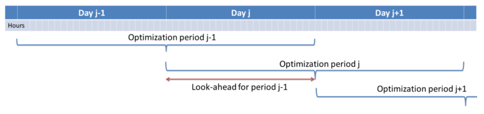
The optimization horizon and overlap period can be adjusted by the user in the Dispa-SET configuration file. As a rule of thumb, the optimization horizon plus the overlap period should at least be twice the maximum duration of the time-dependent constraints (e.g. the minimum up and down times). In terms of computational efficiency, small power systems can be simulated with longer optimization horizons, while larger systems should reduce this horizon, the minimum being one day.

References

[1]

Quoilin, S., Hidalgo Gonzalez, I., & Zucker, A. (2017). Modelling Future EU Power Systems Under High Shares of Renewables: The Dispa-SET 2.1 open-source model. Publications Office of the European Union.

[2]

Quoilin, S., Nijs, W., Hidalgo, I., & Thiel, C. (2015). Evaluation of simplified flexibility evaluation tools using a unit commitment model. IEEE Digital Library.

[3]

Quoilin, S., Gonzalez Vazquez, I., Zucker, A., & Thiel, C. (2014). Available technical flexibility for balancing variable renewable energy sources: case study in Belgium. Proceedings of the 9th Conference on Sustainable Development of Energy, Water and Environment Systems.